#25 PCA for GWAS
Background
Now that we have finalized our matrix table, the final step before releasing our second data release is validating our data with GWAS analysis based on height. In my last blog I mentioned that we were missing some data needed to run GWAS. These included some covariate data, that we are currently waiting for from the VA, and principle components (PCs) generated from PCA analysis. For Data Release 1, PCs were provided by the Boston team. To achieve a more streamlined and automated release process, we set out to implement a PCA pipeline for our final matrix table.
Initial PCA testing for Data Release 1
Although the PC’s used in GWAS analysis for Data Release 1 were not generated in Hail, JIna Song conducted tests shortly after the first data release. These tests are documented in a slide deck. Jina showed that she was able to obtain comparable results using the hail function hwe_normalized_pca when compared to the PCs provided by the Boston team. While the results looked promising, I was unable to locate any the source code or notebook used to generate the data.
Establising a PCA pipeline for GWAS
Over the past few weeks I have worked to develop a PCA pipeline for GWAS, based on the information I learned in Jina’s slide deck. I began by testing the Hail function hwe_normalized_pca to get an idea of how it worked and how to best apply the output to our GWAS methods. In the first test I tried running PCA on our final matrix table. This resulted in an error that is documented here. The Hail team suggested filtering our matrix table for common variants, indicating that between 5,000-10,000 variants might be ideal for running the function.
The methods for ancestry prediction in Data Release 1 incorporated a pipeline that filtered for common variants and then further filtered variants. The steps involved in this pipeline are as follows.
- Filter to include only autosomes
- Filter out non-SNPs
- Filter out variants whose most common allele had a frequency less than 5%
- Prune variants with Hail’s ld_prune algorithm
- Keep remaining variants that overlap with published data in the 1000 Genomes database.
The preceding methods were implemented and 160883 variants remained. PCA was then run on the filtered dataset with success. Steps were then duplicated for each ancestry group to generate a PCs for all groups, i.e., the matrix table was filtered to include only people of Asian descent and then filtered with the 5 steps above.
With PCs now at hand, I was able to begin testing Jina’s height GWAS pipeline. Early results did not show high correlation between theoretical and observed distributions when generating a QQ plot (Fig. 1).
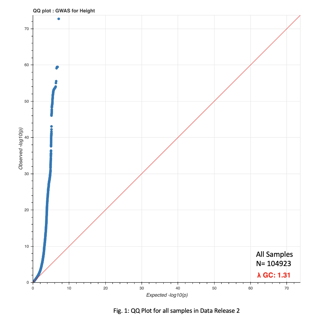
While we are still waiting on age and BMI covariate data, the possibility that my PCA pipeline may need to be revised also exists. While the QQ plot is discouraging, a scatterplot clustering ethnicities based on the first two PCs looks encouraging, and indicates the PCA methodolgy may be valid (Fig. 2).
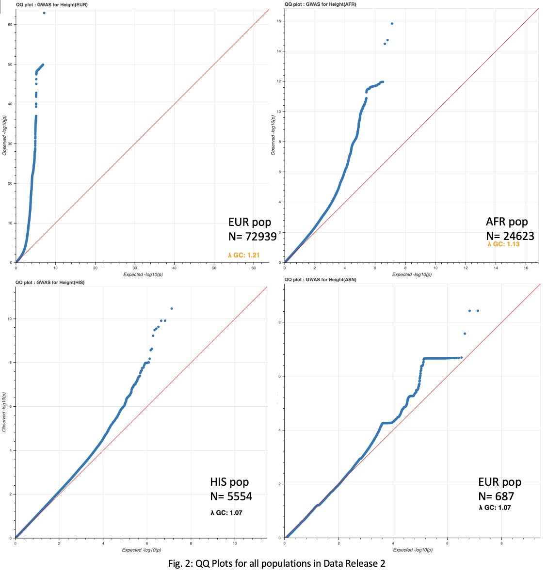
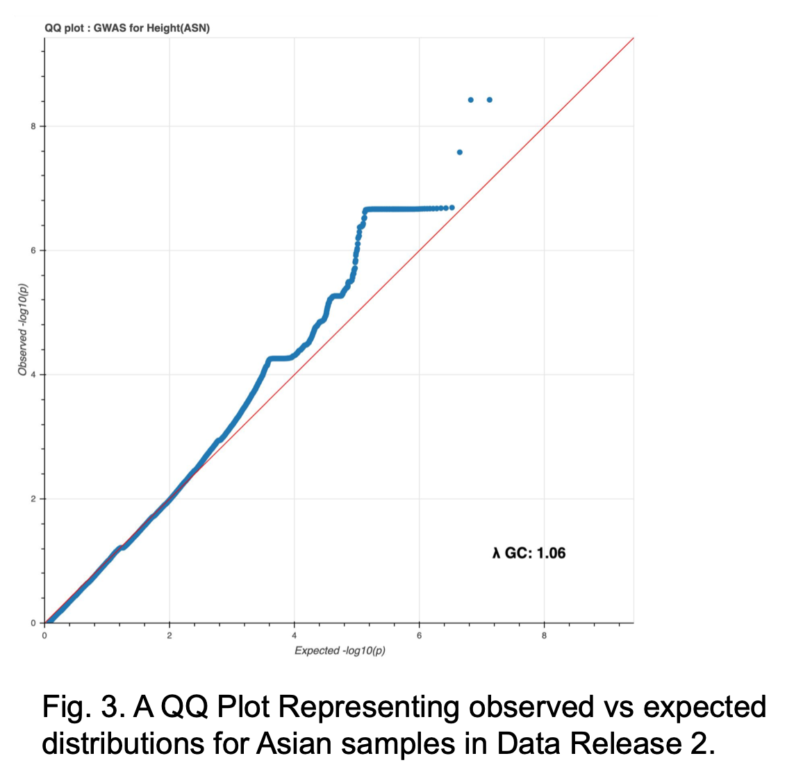
A comparison to Jina’s methods (below) will be made when complete. Additionally, a QQ plot within only Asian populations shows a much better correlation, even without the missing covariates (Fig. 3).
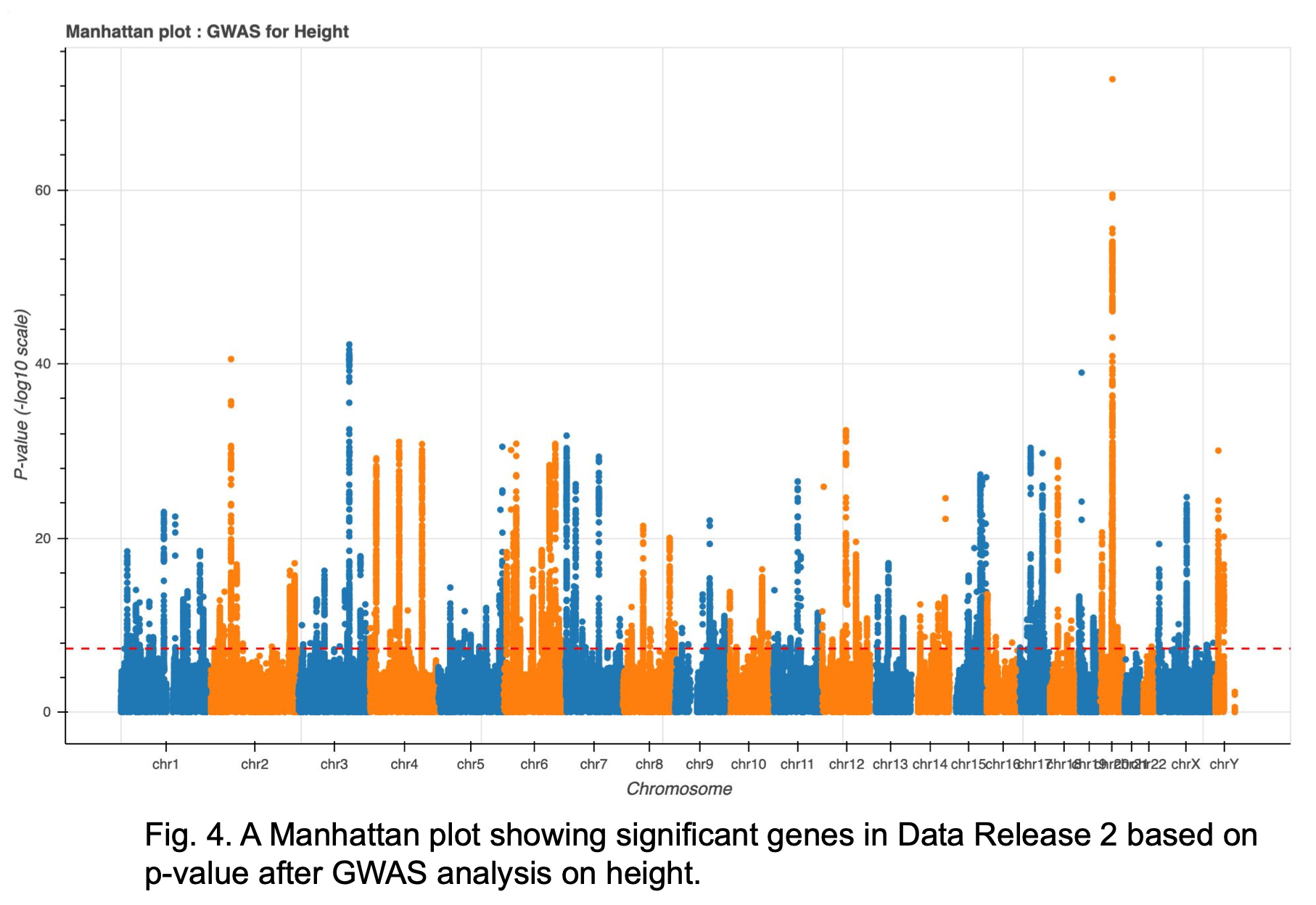
Further investigation is also being done to determine the results of the Manhattan plot (Fig. 4). While the top genes found in Data Release 1 where primarily found on chromosome 7, many of the top results currently found in Rel 2 are on chromosome 20. There is one overlap for top 10 sites at Pos chr20:35437976.
Alternate filtering methods for PCA
After searching through cloud storage, I was able to locate a notebook that contains the information Jina described in her tests. This includes a filtering method for variants prior to PCA. These methods include:
- Filtering variants whose most common allele’s frequency is less than 1%
- Filter to include only autosomes
- Filter out non-SNPs
- Prune with ld_prune
The resulting filters produced a matrix table with roughly 1.5 million variants for the Rel 1 data. This is well above the suggestion of the Hail team, but Jina was able to run PCA and GWAS successfully with this dataset. I am now currently re-running filters on our dataset with Jina’s methods to test GWAS. Additional pieces that may improve GWAS results include incorporating the age and BMI covariates and filtering variants based on minor allele frequency as described in this Hail tutorial.
Discuss
Join the discussion on our GitHub