#33 MVP Release 2 variants #2: Comparing MVP variants to other datasets

Introduction

As part of Data Release 2 of the Million Veteran program whole genome sequencing initiative, Joe created a variant table from Hail, with metadata describing all of the variants we observed. In my last post, I uploaded this table to BigQuery and generated some basic summary statistics. Here, I’ll describe how I’ve continued that effort by doing some preliminary comparative analyses between our dataset and others like 1000 Genomes.

Comparing to 1000 Genomes alternate allele frequency distribution

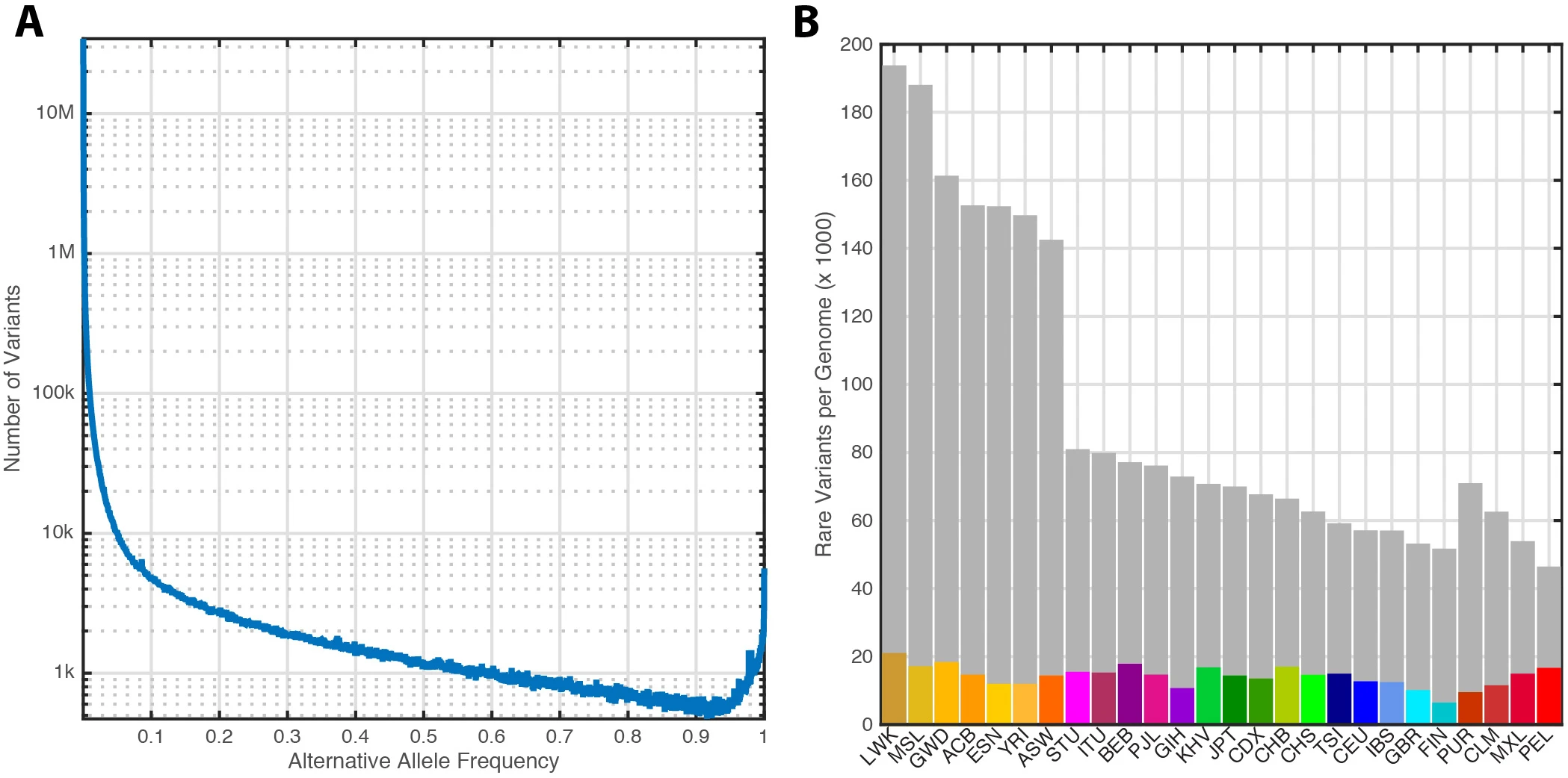Figure 7 from: The 1000 Genomes Project Consortium. A global reference for human genetic variation. Nature 526, 68–74 (2015). https://doi.org/10.1038/nature15393.

Looking at whole genome sequencing publications from other consortiums, I found a lot of sophisticated and complex data analysis that would seemingly require a significant amount of effort to replicate. We will maybe get to those at some point, but I certainly didn’t want to start there. However, the alternate allele frequency histogram only requires one metric (allele frequency) and provides a measure of validation of the “shape” of our data. Here, I’ve tried to replicate it with our data.

SQL query

SELECT
    variant_qc_AF[1] AS alt_allele_freq,
    COUNT(1) AS count
FROM
    `{project_id}.wgs_data_release_2.hail_variant_info`
GROUP BY
    alt_allele_freq
ORDER BY
    alt_allele_freq

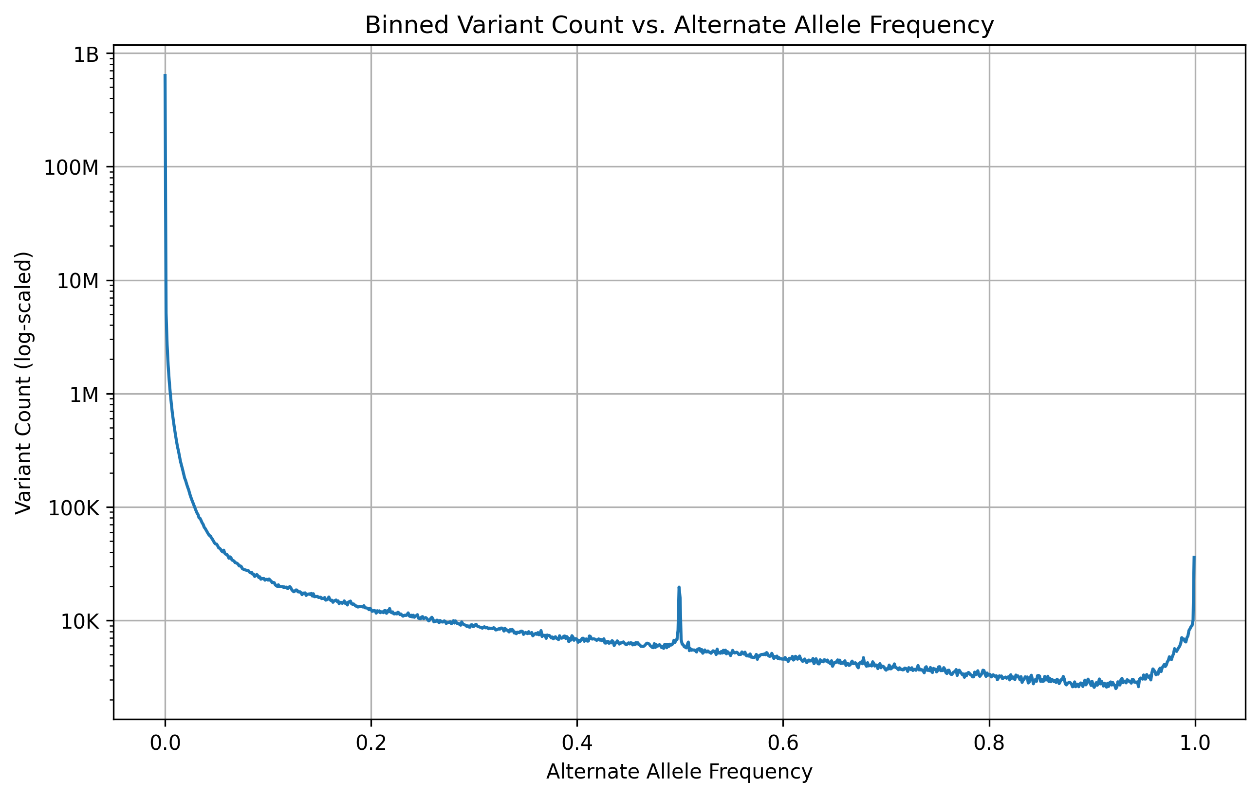
MVP Data Release 2 histogram

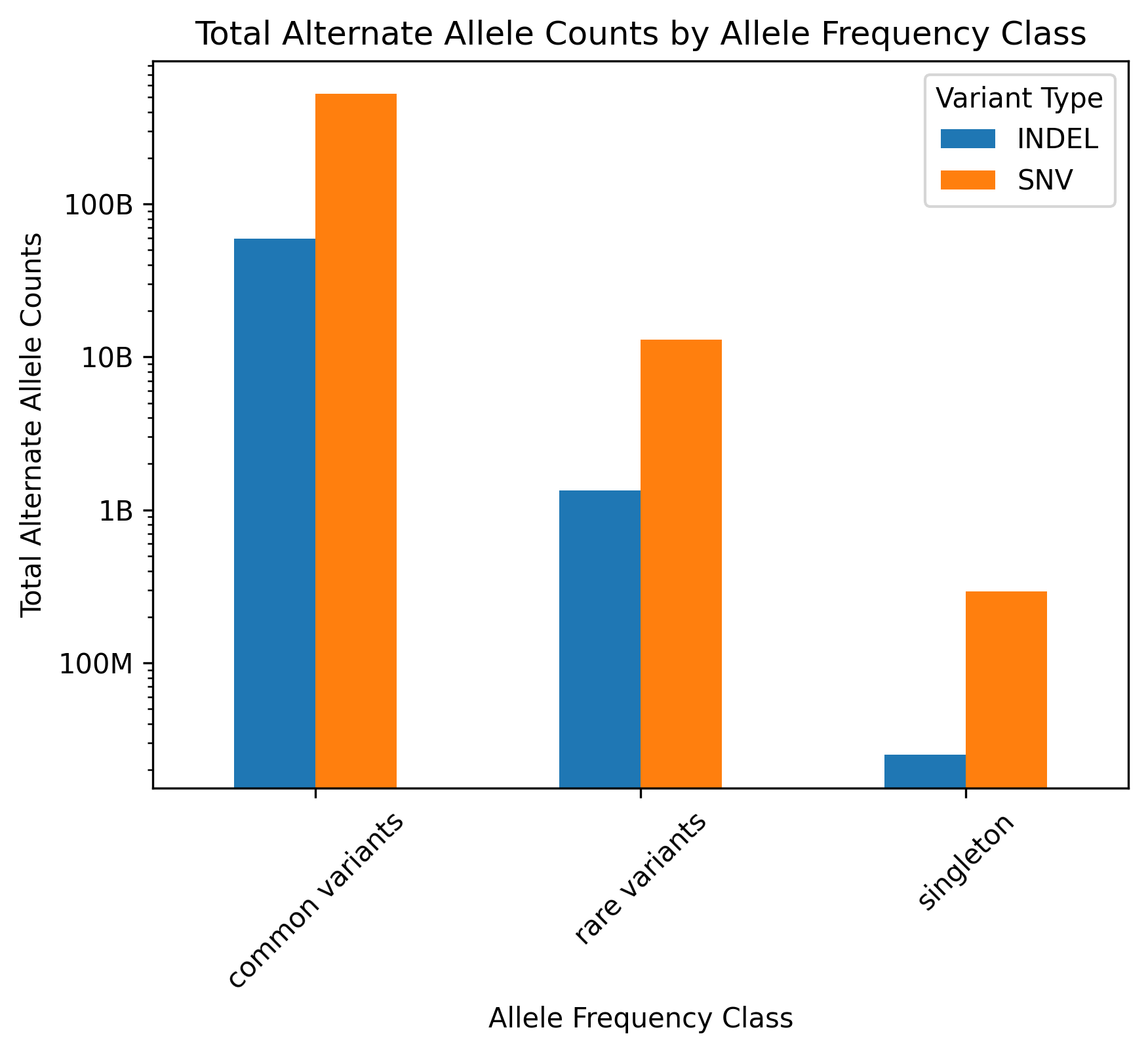
Comparing to 1000 Genomes SNV/Indel counts across frequency categories

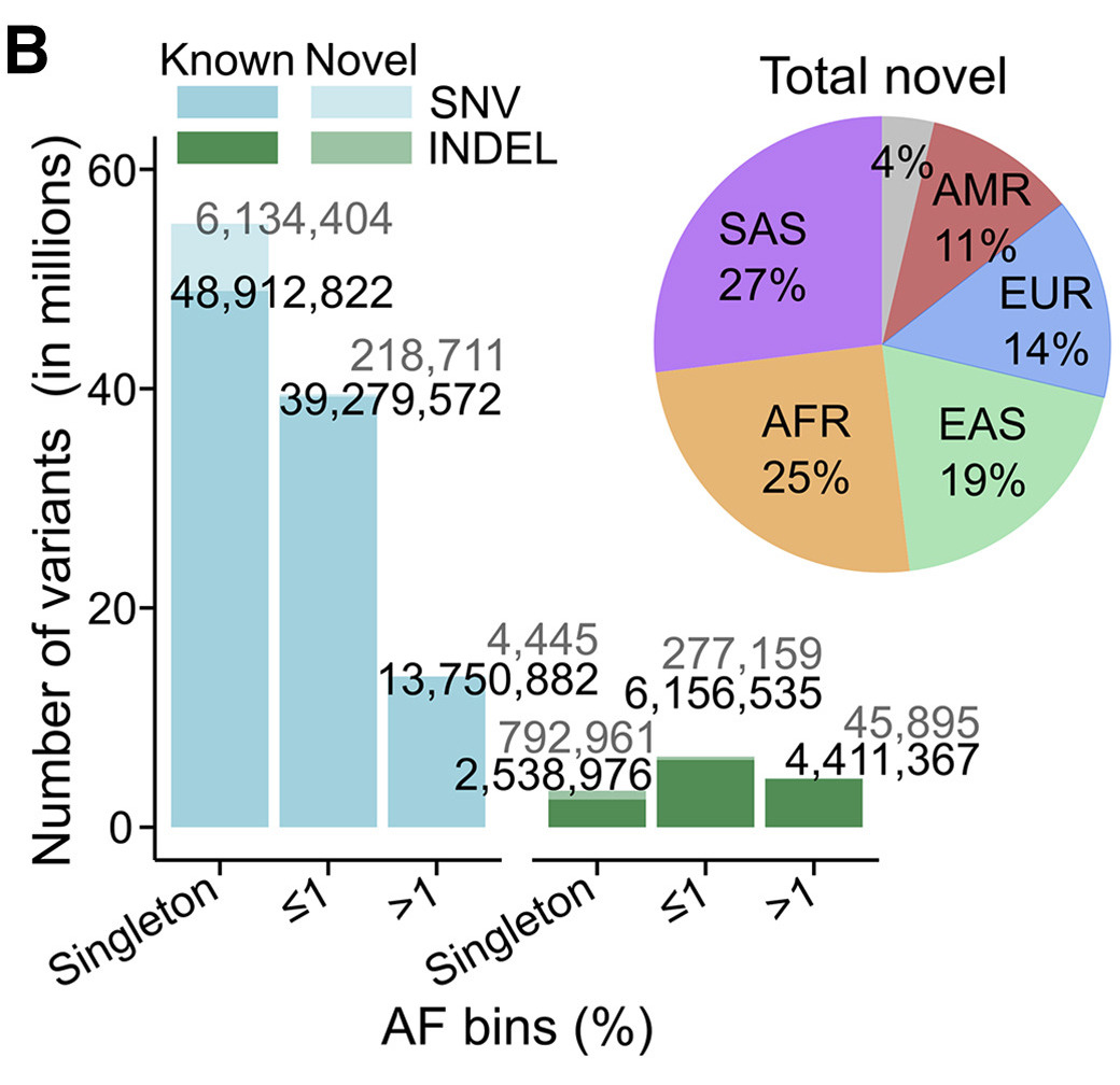Figure 1B from: High-coverage whole-genome sequencing of the expanded 1000 Genomes Project cohort including 602 trios. Cell. 2022 Sep 1;185(18):3426-3440.e19. doi: 10.1016/j.cell.2022.08.004.

In the 1000 Genomes whole genome sequencing publication from 2022, they examine alternate allele counts by type (SNV/INDEL) and frequency bins (singleton, rare, common). I initially thought they were examining number of variants (unique locus and alternate allele combinations), but reading the figure description they indicate that they were looking at “cohort-level alternate allele counts”, so that is what I looked at.

I tried to perform a similar analysis of our data by looking at variant counts (unique locus and alternate allele combinations) as well as alternate allele counts (total number of alternate alleles observed across all variants).

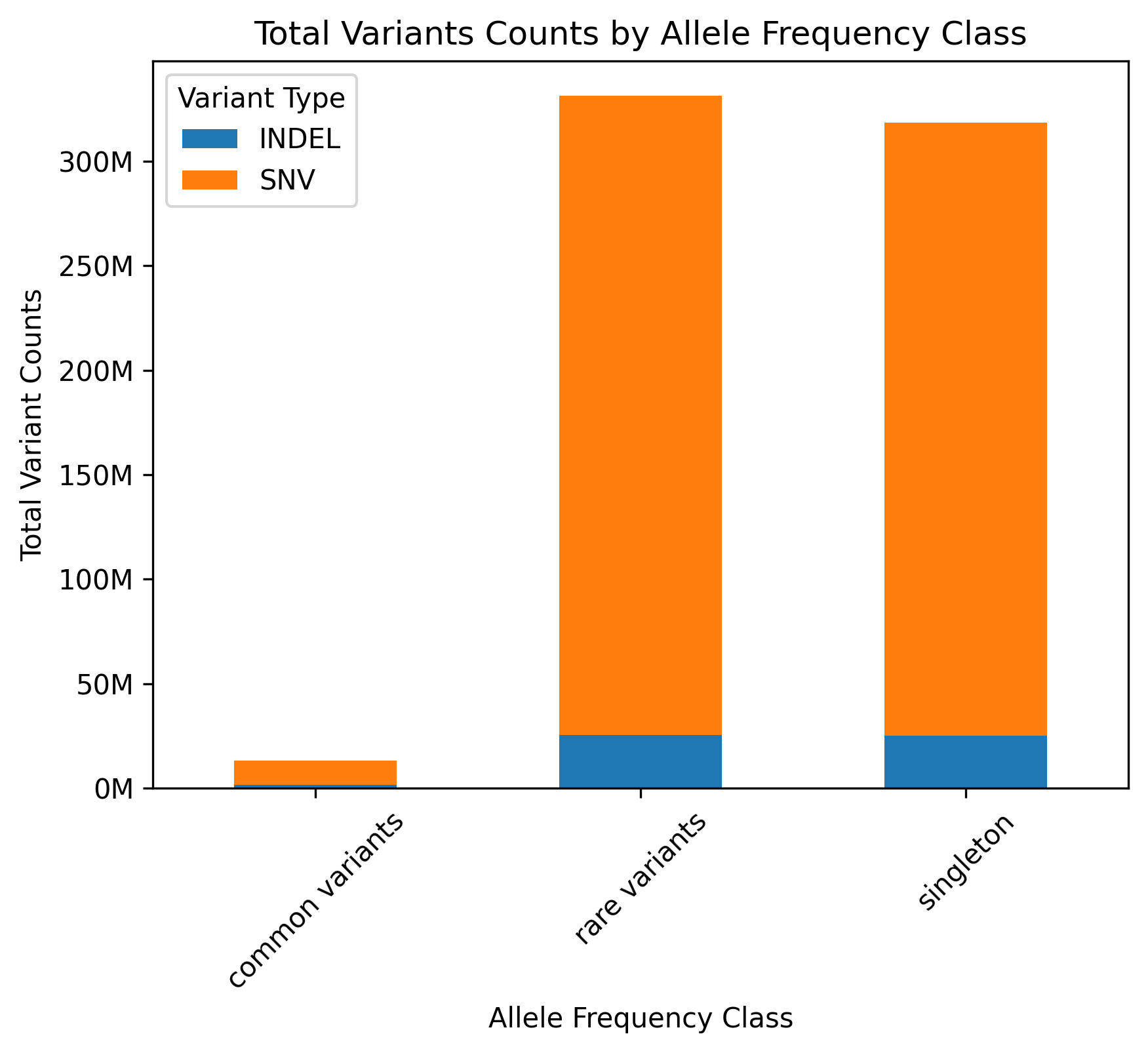
MVP DR2 variant counts by type and frequency category

Here is the plot of variant counts by type and frequency category for MVP Data Release 2. In addition to seeing the breakdown this also provided a validation of my SQL command, because I could check that the total number of variants matched Joe’s reported total.

SQL query

SELECT
    CASE
        WHEN LENGTH(alleles[0]) = 1 
        AND LENGTH(alleles[1]) = 1 THEN 'SNV'
        ELSE 'INDEL'
    END AS variant_type,
    CASE
        WHEN variant_qc_AC[1] = 1 THEN 'singleton'
        WHEN variant_qc_AF[1] <= 0.01 THEN 'rare variants'
        ELSE 'common variants'
    END AS allele_frequency_class,
    COUNT(*) AS total_variant_counts
FROM `{project_id}.wgs_data_release_2.hail_variant_info`
GROUP BY variant_type, allele_frequency_class;

Bar chart

MVP DR2 Alternate allele counts by type and frequency category

A related figure where variant counts have been replaced by alternate allele counts.

Comparing to UK Biobank transition/transversion proportions

In the UK Biobank study they looked specifically at C/T conversions and CG (CpG) -> TG (TpG) converstions because they apparently saw a lot more of these than other possible mutations.

Figure 1a from: Halldorsson, B.V., Eggertsson, H.P., Moore, K.H.S. et al. The sequences of 150,119 genomes in the UK Biobank. Nature 607, 732–740 (2022). https://doi.org/10.1038/s41586-022-04965-x.

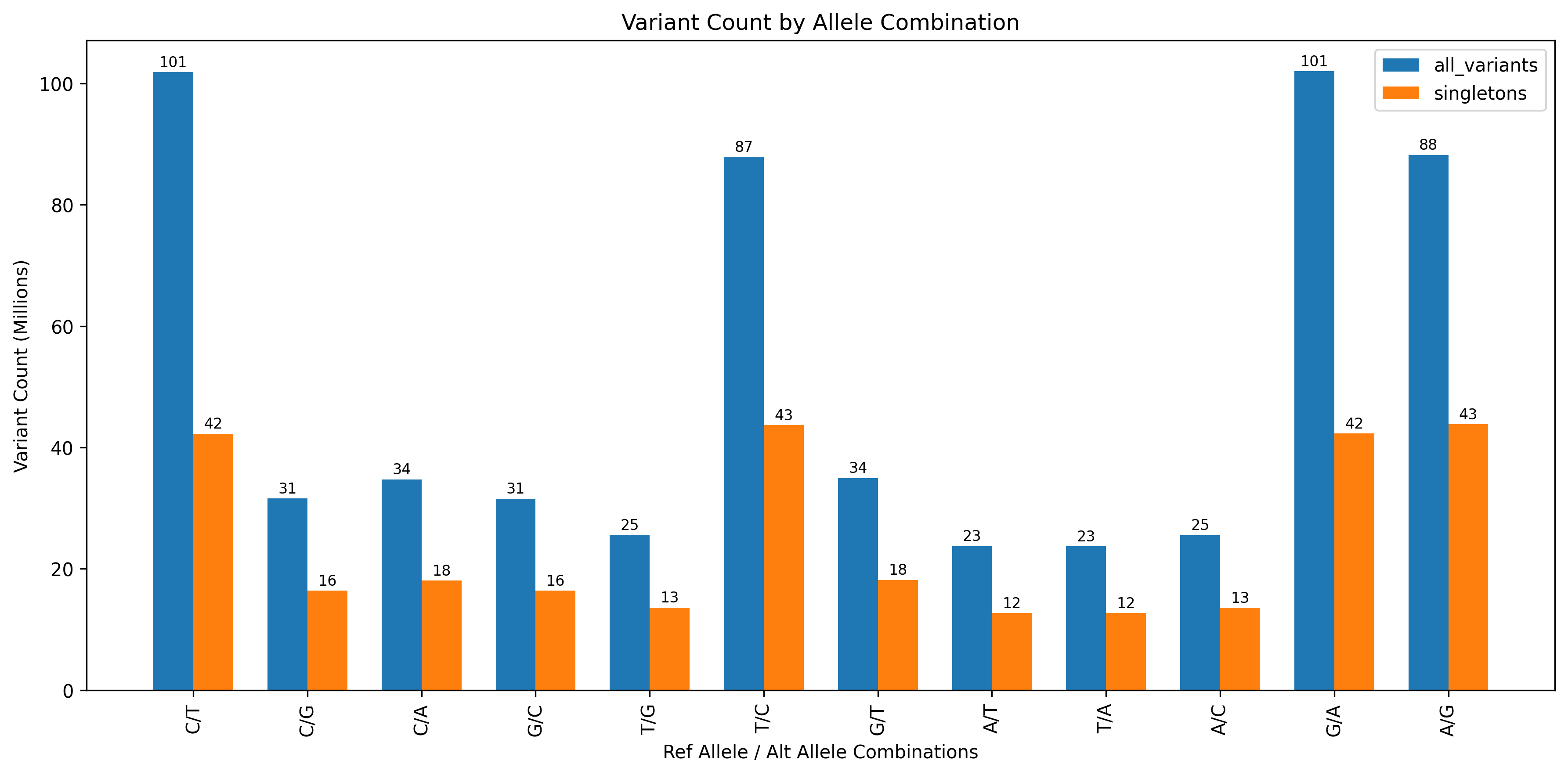
MVP transitions/transversion counts

I performed a similar analysis, but looked at all possible SNV conversions and did not look at dinucleotide pairs such as mutations within CG pairs. I’m also not sure how to do this since I would need to look across rows where the position value is adjacent. But I imagine it’s doable.

SQL query to characterize all single nucleotide changes

SELECT
    alleles[0] AS ref_allele,
    alleles[1] AS alt_allele,
    COUNT(*) AS variant_count
FROM
    `{project_id}.wgs_data_release_2.hail_variant_info`
WHERE
    LENGTH(alleles[0]) = 1
    AND LENGTH(alleles[1]) = 1
GROUP BY
    ref_allele, alt_allele

SQL query to characterize single nucleotide changes among singletons

SELECT
    alleles[0] AS ref_allele,
    alleles[1] AS alt_allele,
    COUNT(*) AS variant_count
FROM
    `{project_id}.wgs_data_release_2.hail_variant_info`
WHERE
    LENGTH(alleles[0]) = 1
    AND LENGTH(alleles[1]) = 1
    AND variant_qc_AC[1] = 1
GROUP BY
    ref_allele, alt_allele

Bar chart

Characterizing short INDELs in MVP DR2

The GATK germline variant calling pipeline calls SNVs as well as small INDELs (insertions and deletions). Structural variants is a particularly active field of research producing increasingly complex workflows involving multiple softwares and machine learning algorithms. I don’t know exactly how GATK calls structural variants, but I’m confident it is not the state of the art. Nevertheless, we already have that data and it seems a waste to just ignore it. Here, I’ve started analyzing INDEL data, by characterizing the lengths of deletions and insertions called by GATK.

The first thing I did was to generate some basic summary statistics. In this case, I’m classifying variants as insertions or deletions based on the relative lengths of the reference and alternative alleles. If the reference is longer than the alternate, I’m calling that a deletion and vice versa. This logic is implemented using a CASE statement. Along with this categorization, I’m also getting the reference and alternate allele length from the variant table, in order to generate my summary statistics. Then I’m calculated min, max, and average values for insertions and deletions.

SQL query

WITH categorized_data AS (
  SELECT
    CASE
      WHEN LENGTH(alleles[0]) > LENGTH(alleles[1]) THEN 'Deletion'
      WHEN LENGTH(alleles[1]) > LENGTH(alleles[0]) THEN 'Insertion'
      ELSE 'Other'
    END AS category,
    LENGTH(alleles[0]) AS ref_allele_length,
    LENGTH(alleles[1]) AS alt_allele_length
  FROM
    `{project_id}.wgs_data_release_2.hail_variant_info`
)

SELECT
  category,
  COUNT(*) AS count,
  AVG(ref_allele_length) AS avg_ref_allele_length,
  AVG(alt_allele_length) AS avg_alt_allele_length,
  MIN(ref_allele_length) AS min_ref_allele_length,
  MIN(alt_allele_length) AS min_alt_allele_length,
  MAX(ref_allele_length) AS max_ref_allele_length,
  MAX(alt_allele_length) AS max_alt_allele_length
FROM
  categorized_data
WHERE
  category IN ('Insertion', 'Deletion')
GROUP BY
  category;

SQL result

category	count	avg_ref_allele_length	avg_alt_allele_length	min_ref_allele_length	min_alt_allele_length	max_ref_allele_length	max_alt_allele_length
Insertion	16450545	1.00000	7.712097	1	2	1	667
Deletion	35550084	5.21684	1.000000	2	1	364	1

Just from the summary statistics I can see that it looks like insertions are generally longer than deletions and that most INDELs are small; less than 10 base pairs. To better understand the shape of the data I also wanted to plot the distribution of lengths using a histogram. To gather this data, I ran another SQL query to generate counts of each observed INDEL length, grouped by structural variant category.

SQL query

WITH categorized_data AS (
  SELECT
    CASE
      WHEN LENGTH(alleles[0]) > LENGTH(alleles[1]) THEN 'Deletion'
      WHEN LENGTH(alleles[1]) > LENGTH(alleles[0]) THEN 'Insertion'
      ELSE 'Other'
    END AS category,
    LENGTH(alleles[0]) AS ref_allele_length,
    LENGTH(alleles[1]) AS alt_allele_length
  FROM
    `{project_id}.wgs_data_release_2.hail_variant_info`
)

SELECT
  category,
  COUNT(*) AS count,
  ABS(ref_allele_length - alt_allele_length) AS indel_length
FROM
  categorized_data
WHERE
  category IN ('Insertion', 'Deletion')
GROUP BY
  category, ref_allele_length, alt_allele_length;

SQL result

Here are the first (5) lines of the dataframe I generated from that query, to give you an idea what the results look like.

category	count	indel_length
Deletion	176	209
Insertion	86	184
Insertion	6	253
Deletion	194	240
Deletion	1	350

Histogram of MVP INDEL lengths

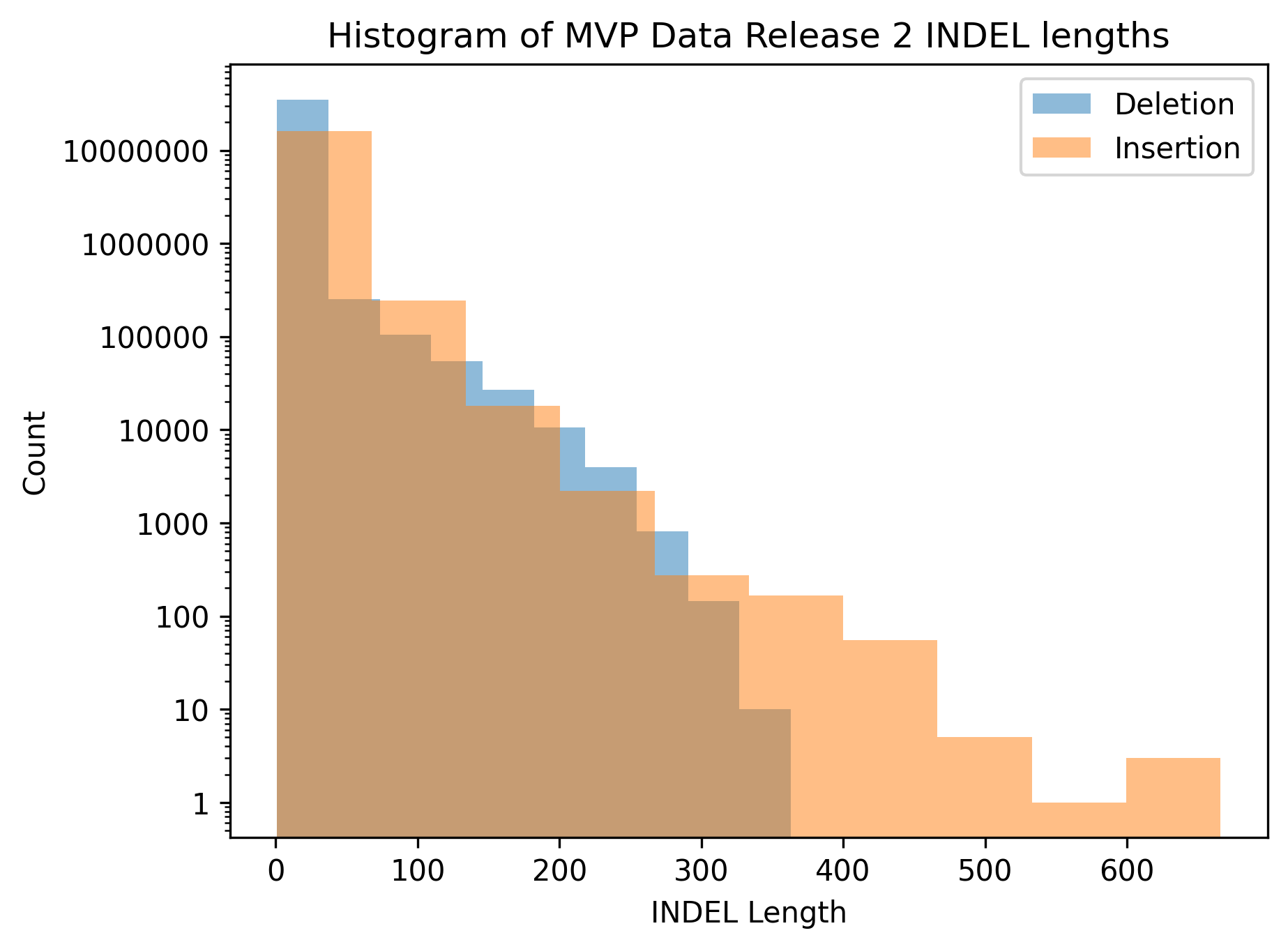
And here is a histogram generated from that data. I think something worth keeping in mind when looking at the histogram is that while it’s sometimes nice to have a visualization to look at, it took significantly more effort to generate the figure than it did to generate the summary statistics, and we didn’t gain much information. Of course, I didn’t know that before doing the exercise, and we may have seen something like a bimodal distribution that wouldn’t have been apparent just looking at min/max/average.

Future directions

The notebook I used to perform these analyses is available internally on GitHub. Feel encouraged to check it out even though it is still in a somewhat raw state. I also peformed a few more analyses using Ensembl gene annotations I uploaded to BigQuery. You can see where I looked at the number of observed variants in different functional regions for particular genes. I tried running a similar query to calculate the same metrics across all genes, but that either got stuck or takes a very long time to run. Which I think makes sense given that there are ~20,000 genes with 50 different functional regions and to determine whether a variant is in a region, you have to compare the position to the start and end sites of the gene. Regardless, I’m looking forward to doing more gene based analyses of our variant data in the future.

Discuss

Join the discussion of this post on GitHub!