Whole Genome Sequencing Data Release 2 Process Summary

Sequencing and Variant Calling

Whole Genome Sequencing (WGS) for each individual, conducted by Personalis, was delivered to MVP in fastq format. We aligned the sequenced reads using BWA-MEM and called variants using HaploypeCaller, following the recommended best practices described by the Broad Institute. Scripts for alignment and variant calling can be found here. Prior to aggregation, gVCF files were required to pass several QC metrics before proceeding (Table 1). Out of 127,039 gVCF files, 109,726 had passed our QC filters and could proceed to aggregation. While we filtered out around 14% of our samples, many of them were not filtered out due to poor quality but rather not having QC statistics associated with them. Details of how many samples were filtered at each step can be found in this notebook. We will need to Investigate why some samples did not have associated QC statistics for subsequent releases.

Table 1. Summary of pre-aggregation QC criteria

Stage	Tool	Version	Input	QC Description
Raw Sequenced Reads	FastQC	0.11.4	fastq	Average base sequence quality of 28 or greater
Raw Sequenced Reads	FastQC	0.11.4	fastq	Average GC content between 40 and 41%
Sequence Alignment	samtools	0.1.19	BAM	Properly paired read percentage of 95 or greater
Sequence Alignment	verifyBAMID		BAM	Contamination rate of less than 5%

Aggregation

For Data Release 1 we had aggregated around ten thousand samples using the run_combiner() tool provided by Hail. We began to incur spark memory issues while scaling up for the current data release. We then set out to aggregate our samples into batches of ten thousand, which would then be re-aggregated into a larger grouping. These batches took the gVCF files directly as input, resulting in Hail sparse matrix tables (SMT) of ten thousand samples. We then used these SMT batches as input to aggregate into the larger SMT, theoretically using less memory than gVCF files as input. Unfortunately, spark was not able to handle the load.

We then implemented a new method developed by the Hail team. The new method aggregates the samples into a Variant Dataset (VDS), in place of an SMT. VDS aggregation presents a new method that is both more time and memory efficient than SMT aggregation. VDS functionality also allows for seamless transition between VDS and SMT. This allowed us to convert our aggregated table to SMT for downstream analysis.

vds.new_combiner() allows for gVCF or VDS as input. Because we had several batches of ten thousand sample SMTs, and SMTs can easily be converted into VDS, we converted all our SMTs into VDS and proceeded to aggregate them. The resulting table consisted of 109,826 samples and 2,909,379,928 bases. It should be noted that 102 of these samples were the result of sample duplication, resulting in an increase in the 109,726 samples from our QC step. We removed these samples in a processing step downstream that removes all sample duplicates.

Quality Control

To provide quality variants to the MVP community, we set forth a stringent QC filtering pipeline for the aggregated data. Because the methodology is not compatible with VDS, we first converted the aggregated table into SMT format. We next pre-processed the data by removing blacklist regions as specified by ENCODE, removing low complexity regions, and splitting multiallelic sites into individual variant rows. We then assessed the data for quality at three levels: genotype, variant, and sample.

Genotype Level QC

We conducted genotype level quality control for the following conditions:

All Genotypes
- Must have a depth of 400 or less to be retained.
- Must have a depth of 10 or greater except those within male sex chromosomes which have a depth cut off of 5.
Alleles that are homozygous for the reference allele
- Must have a genotype phred quality score of 20 or more
- Note: All homozygous reference alleles are filtered out, making this step redundant.
Alleles that are homozygous for the alternate allele
- Must have an alternate allele frequency of 90% or greater.
- Must have a phred-scaled likelihood ratio of 20 or greater.
- Must have a reference allele frequency of 50% or less and a genotype quality phred score or 20 or more.
Heterozygous genotypes
- Must have a phred-scaled likelihood ration of 20 or greater.
- Must have an alternate allele depth that is at least 20% of the total allele depth.
- The alternate alle depth and reference allele depth must sum to at least 90% of the total allele depth.

Variant Level QC

For variant level QC we first began by annotating each sample with ancestry prediction. This allowed us to calculate and store Hardy-Weinberg equilibrium (HWE) P-Values for each population group at each variant. We then annotated each variant with a pass or fail binary condition. Passing variants were dependent on the population group with the lowest HWE P-Value for that locus. Variants that passed contained a HWE P-Value being at least 1e-5 with a minor allele frequency greater than 1% or the HWE P-Value being 1e-6 with a minor allele frequency of 1% or less. We stored the binary pass/fail condition as metadata for the corresponding variant, but we did not factor it into variant filtering. We next checked that each variant had an alternate allele count of at least one before removing all variants with a call rate of less than 80%.

Sample Level QC

We filtered out samples that did not meet quality standards for two QC metrics. First, we removed any samples with a call rate of less than 97%. Second, we retained only those samples with mean depth greater than 18.

Final Processing and File Generation

After QC filtering we prepared the matrix table for release with final processing and file generation. We first checked that no sample duplicates remained in the matrix table. We next annotated samples in the matrix table with a binary flag depending on whether they have a first- or second-degree relationship, as determined by MVP genotype array data. In the last processing step we removed all samples in the matrix table that did not have a corresponding match in an additonal list of samples to retain. This additonal list was provided to us by the Boston team, consists only of samples that are included in the genotype array data, and omits any samples known to be technical duplicates. A summary of all data output at each processing step described is included below (Table 2).

Table 2. Output of data processing step by step

Process	File Type	Size	Samples	Bases	% Genotypes Filtered
Aggregated Table	VDS	260.35Tib	109,826	2,909,379,298	NA
Pre-processed Table	SMT	279.53TiB	109,826	919,057,644	NA
QC’d Table	SMT	194.73TiB	108,171	663,351,127	5.41%
Final Matrix Table	SMT	188.86TiB	104,923	663,351,127	NA

Once the matrix table was finalized, we exported the data as several file types (Table 3). The only file that currently is released to the public is the genotype information that is contained in a VCF file consisting of 104,923 samples and 663,351,127 variants. This file is converted to a PGEN file by the Boston team to load for MVP researchers.

Table 3. Files generated from final data table

Data	File Type	Size	Compressed	Split By Chromosome	Released to MVP Community
All Data	Hail matrix table	188.86 TiB	NO	NO	NO
Variant Statistics	text	31.5 GB	YES	NO	NO
Sample Statistics	text	25. 7MB	NO	NO	NO
Genotype Data	VCF	1.6 TB	YES	NO	NO
Genotype Data	BGEN	1.3 GB-20.3 GB	NO	YES	NO
Genotype Data	PGEN			NO	YES

Validation

GWAS on Height

Correlation to Data Release 1

Validation of data is crucial to any major study. For Data Release 1, we observed the correlation between European GWAS on height with that of the of MVP’s genotype array data. Having validated the data of Data Release 1, we set out to validate our current dataset by comparing European GWAS on height across both datasets. We processed the samples in the current release with the GWAS pipeline as described and used in Data Release 1. For reference, this pipeline consisted of the following steps:

Common variants are filtered using an allele frequency cutoff of 1% of for the alternate allele.
The population group of interest is pulled out by filtering samples based on ancestry prediction.
GWAS on height is calculated with a linear regression algorithm in Hail with the following covariates
- Sex
- Age
- Age Squared
- BMI
- First 10 principal components calculated from genotype array data for the specified population group

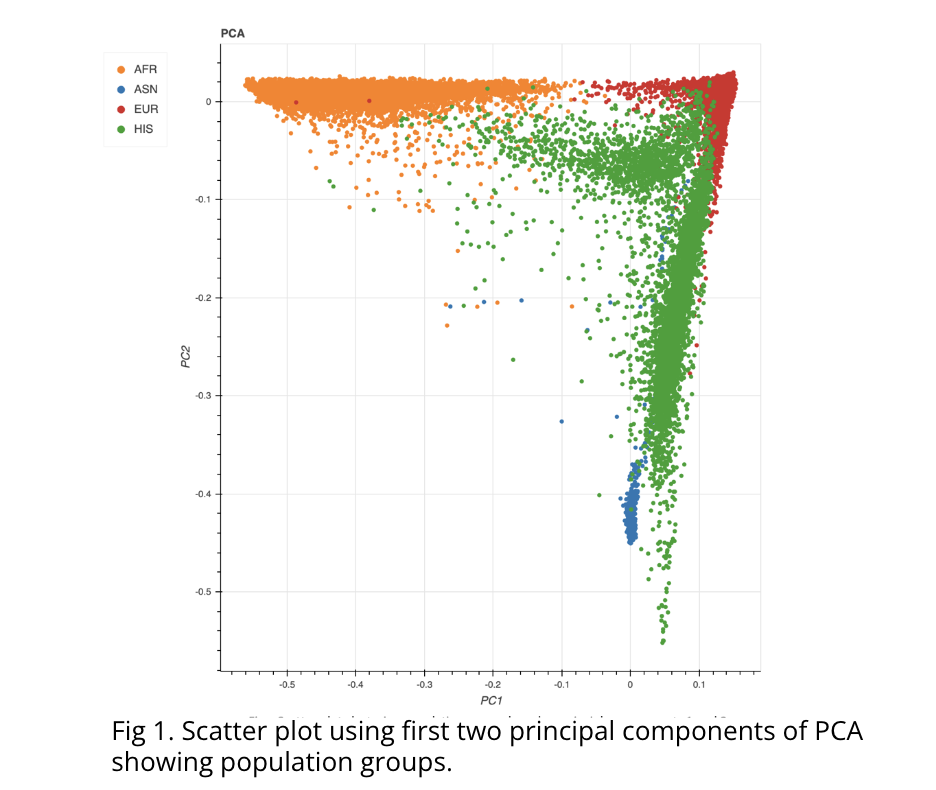
For a consistent correlation study, we followed this pipeline with some key differences. Because age and BMI information was not made available to us, these covariates were omitted from our GWAS study. Additionally, while principal components (PCs) from Data Release 1 were obtained from PCA analysis of the aforementioned genotype array data, we developed a new PCA pipeline to generate PCs based on the WGS data, using Hail. Results of our PCA showed clear separation of samples based on their ethnicity (Fig 1). To obtain the best correlation, we also downsampled to include only samples within Data Release 1. This resulted in 10,385 total samples, before removing non-Europeans, compared to the 10,390 that were processed in the first release.

Fig. 1

Results of the correlation study showed high correlation between both GWAS results. Pearson and Spearman correlation coefficients showed scores of .959 and .927, respectively, indicating very strong correlation. Additionally, we sorted the variants from each study’s GWAS results by P-Value. 92 of the top 100 loci were found to be matched in both studies.

Results from Data Release 2

With our data showing high correlation with that of the first data release, we wanted to explore our current data further. We chose to perform GWAS on height for our African American population because this population contained the most variants and because it is an underutilized group in genomic studies. For GWAS on the current data set, we changed two steps in our pipeline from that of the first data release. First, we filtered for common variants in individual populations as opposed to a universal filter. Second, we applied LD Pruning to the GWAS results. The pipeline we are currently using looks like this:

The population group of interest is pulled out by filtering samples based on HARE data.
Common variants are filtered using an allele frequency cutoff of 1% for the alternate allele.
GWAS on height is calculated with a linear regression algorithm in Hail with the following covariates
- Sex
- First 10 principal components calculated for the specified population group
GWAS results are pruned with the LD prune function in Hail

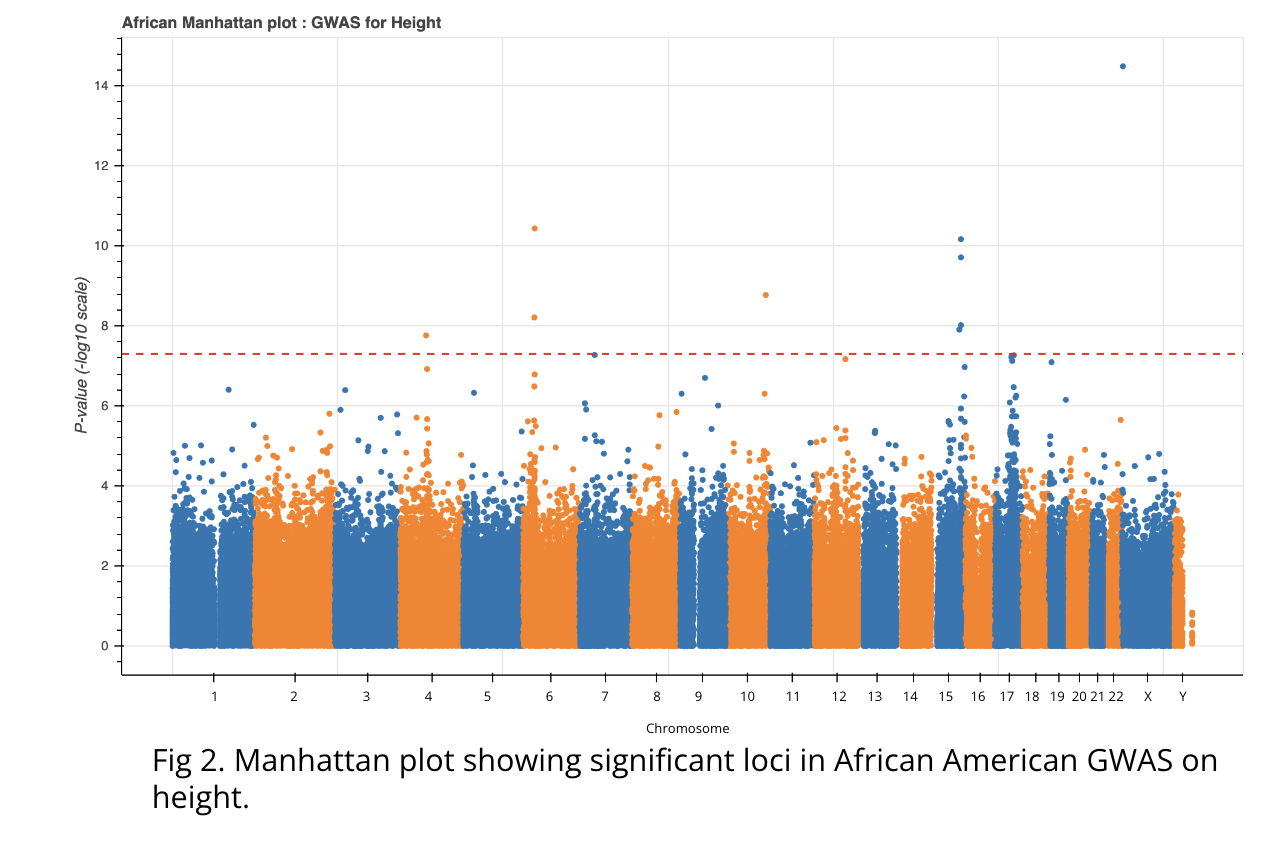
GWAS on height, in the African American population, resulted in nine significant variants (Fig 2). We annotated the corresponding loci using VEP and Biomart. Eight of the nine loci resided within six genes, TCP11, FRAS1, ADAMTSL3, ARSL, ACAN, and NUDT3, with one variant 10kb upstream of FGFR2, all of which have known height associations in the EBI and GeneCards databases. Additionally, three of the candidate variants and all seven associated genes have previously been described as being associated with height regulation in African Americans (Carty et al., N’Diave et al., Yengo et al.), further validating our data.

Fig. 2

Burden Testing

Novel Variant Discovery

Join the discussion here!