Overview

We have been working on a few different analysis to help validate the results that we got from running TelSeq on the MVP genomes. In this specificUK BioBank study they have described an interesting method to predict age using the estimated leukocytye telomere length.

To quote the authors:

“To assess performance for single and combined telomere length metrics we randomly sampled 10,000 participants from the full dataset. We used this training set to fit a simple linear model of a given telomere length metric with age (that is, age ~ telomere lengthmetric). Then, using the held-out participants, we used the model to predict age and assessed prediction performance as the root mean squared error of the age predictions. To perform crossvalidation and obtain CIs for these performance estimates, we performed this procedure 100×, sampling with replacement”

1. Implementation of the prediction model

We will use a linear regression model to predict age based on leukocyte telomere length.

Random Sampling: We will randomly select a subset of 10,000 participants from our dataset for each iteration. This will help ensure that our model is robust and not overly fitted to any specific subset of data.
Model Fitting: For each sampled group, we will fit a simple linear regression model, where the independent variable is leukocyte telomere length and the dependent variable is age. This model will help us understand the relationship between telomere length and age.
Making Predictions: Once the model is fitted, we will use it to predict the ages of the participants in the sampled dataset. These predictions will be compared against the actual ages to assess the model’s performance.
Calculating RMSE: For each iteration, we will calculate the Root Mean Square Error (RMSE), which quantifies the average difference between the predicted ages and the actual ages. RMSE is a valuable metric as it gives us insight into how well the model performs in predicting age based on telomere length.
Cross-Validation: We will repeat this entire process 100 times, each time with a different random sample. This cross-validation approach allows us to evaluate the model’s performance across various subsets of data and helps mitigate any potential bias introduced by a particular sample.
Confidence Intervals: After obtaining RMSE values from all 100 iterations, we will calculate confidence intervals for these RMSE values. This will provide us with a range within which we can be confident that the true RMSE lies, allowing us to better understand the variability and reliability of our model’s predictions.

import statsmodels.api as sm
from sklearn.metrics import mean_squared_error
from sklearn.utils import resample
import numpy as np

# Define parameters for cross-validation
n_iterations = 100  # Number of iterations for sampling and model fitting
n_samples = 10000   # Number of samples to draw in each iteration
rmse_list = []      # List to store RMSE values from each iteration

# Loop through the specified number of iterations
for _ in range(n_iterations):
    # Sample the dataset with replacement to create a bootstrap sample
    sample = resample(
        wgsdr2_ltl_gia_104k_na_removed_from_age_sex_gia_eur_afr_amr_lt_80,
        n_samples=n_samples,
        replace=True  # Enable replacement for bootstrap sampling
    )

    # Fit the linear regression model using the bootstrap sample
    X = sm.add_constant(sample['LENGTH_ESTIMATE'])  # Add a constant for the intercept
    model = sm.OLS(sample['age_blooddraw'], X).fit()  

    # Identify the held-out participants (those not included in the sample)
    held_out = wgsdr2_ltl_gia_104k_na_removed_from_age_sex_gia_eur_afr_amr_lt_80[
        ~wgsdr2_ltl_gia_104k_na_removed_from_age_sex_gia_eur_afr_amr_lt_80.index.isin(sample.index)
    ]

    # Prepare the features for prediction on the held-out set
    X_held_out = sm.add_constant(held_out['LENGTH_ESTIMATE'])  # Add intercept

    # Make predictions on the held-out data using the fitted model
    predictions = model.predict(X_held_out)

    # Calculate the Root Mean Square Error (RMSE) between actual and predicted ages
    rmse = np.sqrt(mean_squared_error(held_out['age_blooddraw'], predictions))
    rmse_list.append(rmse)  # Store the RMSE for this iteration
    
# After all iterations, calculate the mean RMSE across all samples
mean_rmse = np.mean(rmse_list)

# Calculate the 95% confidence intervals for the RMSE
# The 2.5th and 97.5th percentiles provide the bounds for the confidence interval
conf_interval = np.percentile(rmse_list, [2.5, 97.5])

# Print the results: mean RMSE and the 95% confidence interval
print(f'Mean RMSE: {mean_rmse}')
print(f'95% Confidence Interval: {conf_interval}')

Prediction results

Mean RMSE: 10.423690470669865
95% Confidence Interval: [10.39575028 10.44459771]

Mean RMSE: The root mean squared error (RMSE) of 10.42 indicates the average difference between the predicted ages and the actual ages across your held-out participants. An RMSE value gives you a measure of how well your model predicts age; lower values indicate better predictive accuracy.
In this context, a mean RMSE of 10.42 means that, on average, the model’s predictions of age are about 10.42 years off from the actual ages.
The 95% confidence interval for the RMSE, which ranges from 10.40 to 10.44, suggests that you can be 95% confident that the true mean RMSE of your model, if you were to run this analysis multiple times, would fall within this range.
This narrow interval indicates that your RMSE estimate is quite stable, meaning that the performance of your model is consistent across different random samples.

To conclude - The mean RMSE of about 10.42 suggests that the model has a moderate level of accuracy in predicting age based on telomere length.

2. Performing a univariate analysis (as shown in the study) to understand the effect of estimated LTL on age

A univariate analysis examines the relationship between a single independent variable (predictor) and a dependent variable (outcome). In this case, we will analyze how leukocyte telomere length predicts age.

import statsmodels.api as sm

# 1. Fit the univariate linear model
X = wgsdr2_ltl_gia_104k_na_removed_from_age_sex_gia_eur_afr_amr_lt_80
    ['LENGTH_ESTIMATE']  # Predictor
y = wgsdr2_ltl_gia_104k_na_removed_from_age_sex_gia_eur_afr_amr_lt_80
    ['age_blooddraw']  # Response

# Add a constant (intercept) to the model
X = sm.add_constant(X)

# Fit the model
univariate_model = sm.OLS(y, X).fit()

# Print the summary of the model
print(univariate_model.summary())

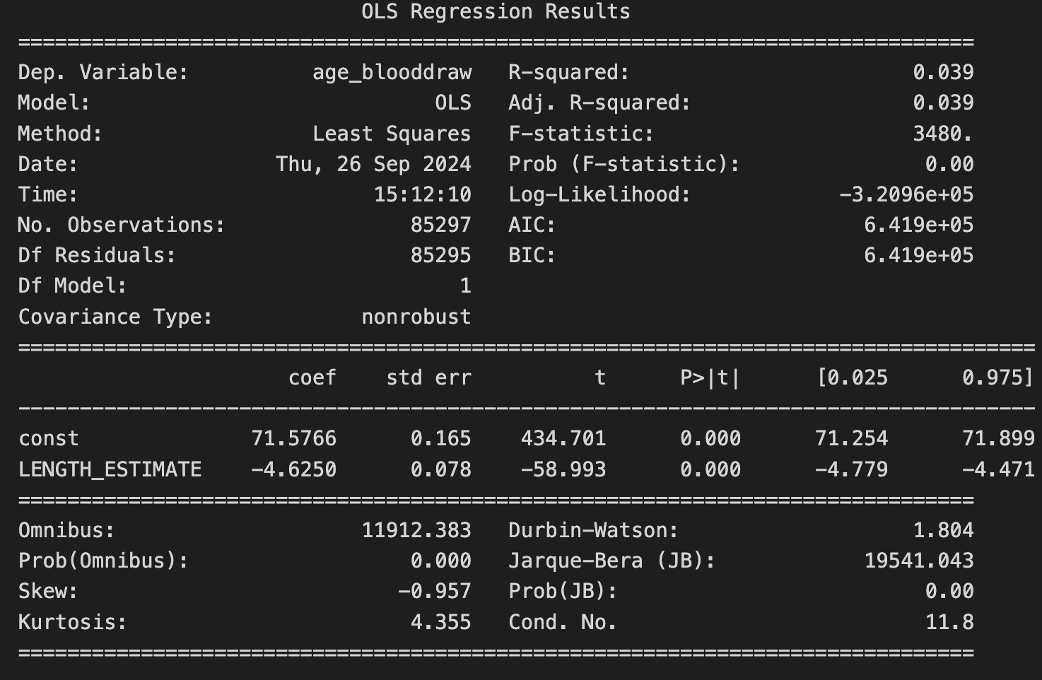
Results:

The model indicates a statistically significant negative relationship between telomere length and age, suggesting that individuals with longer telomeres tend to be younger.
However, the low R-squared value (0.039) indicates that while there is a significant relationship, LENGTH_ESTIMATE alone does not explain much of the variability in age. Other factors likely contribute to age, and further analysis incorporating additional variables might provide a more comprehensive understanding.

#2. Predict age using the fitted univariate model
# Using the LENGTH_ESTIMATE values from the original DataFrame
predictions = univariate_model.predict(X)

# Add predictions to the original DataFrame
wgsdr2_ltl_gia_104k_na_removed_from_age_sex_gia_eur_afr_amr_lt_80
    ['Predicted_Age'] = predictions

# 3. Generate a Bland-Altman plot
# Calculate mean and difference
mean_age = (wgsdr2_ltl_gia_104k_na_removed_from_age_sex_gia_eur_afr_amr_lt_80
    ['age_blooddraw'] + predictions) / 2
diff_age = predictions - wgsdr2_ltl_gia_104k_na_removed_from_age_sex_gia_eur_afr_amr_lt_80['age_blooddraw'] 

# Calculate limits of agreement
mean_diff = np.mean(diff_age)
std_diff = np.std(diff_age)
lower_limit = mean_diff - 1.96 * std_diff
upper_limit = mean_diff + 1.96 * std_diff

# Create the Bland-Altman plot
plt.figure(figsize=(10, 10))
plt.scatter(mean_age, diff_age, alpha=0.5)
plt.axhline(mean_diff, color='gray', linestyle='--', label='Mean Difference')
plt.axhline(lower_limit, color='red', linestyle='--', label='Lower Limit of Agreement')
plt.axhline(upper_limit, color='blue', linestyle='--', label='Upper Limit of Agreement')
plt.title('Bland-Altman Plot - ')
plt.xlabel('Mean Age')
plt.ylabel('Difference between Predicted and Actual Age')
plt.legend()
plt.grid()
plt.show()

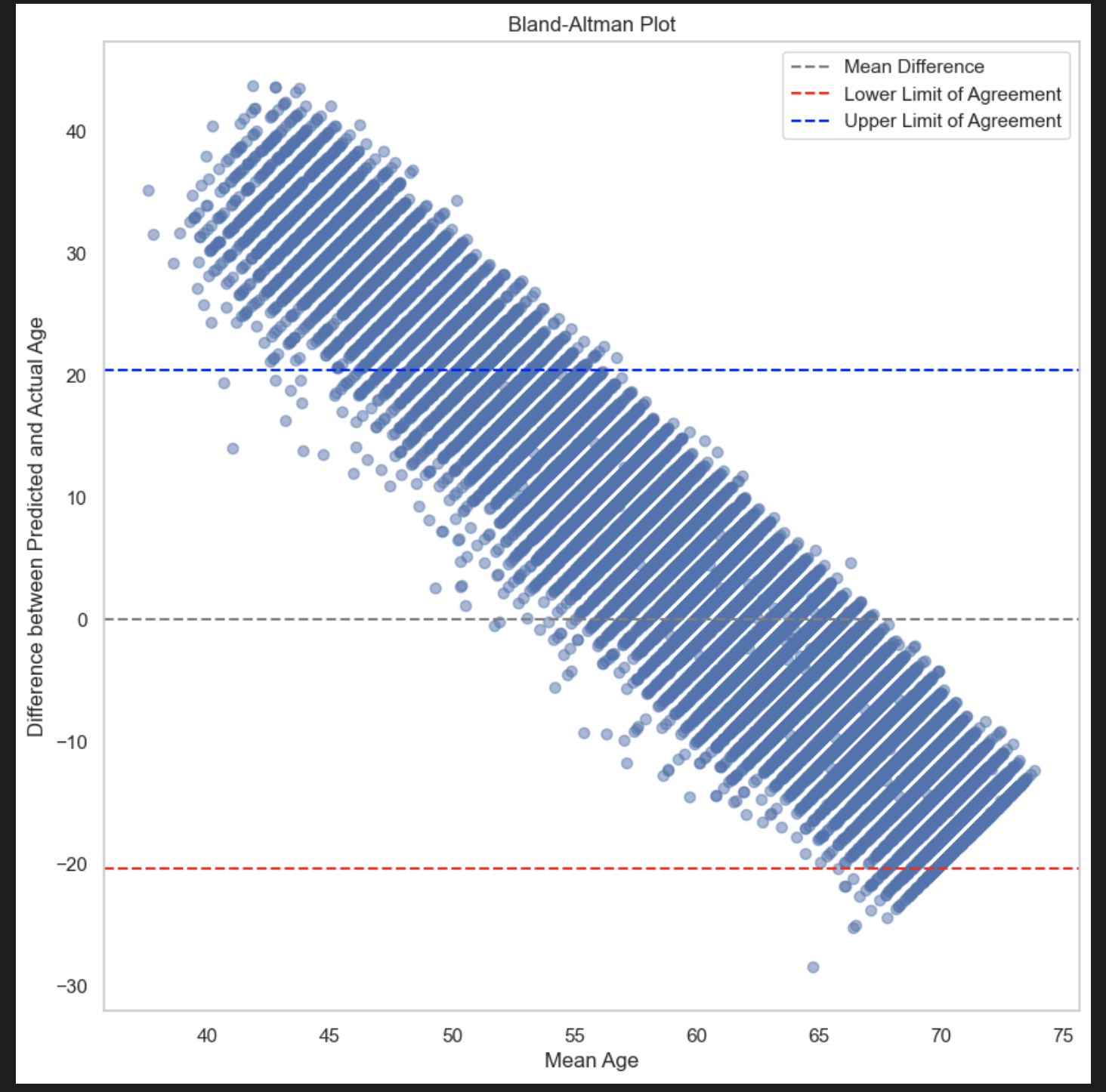
Results:

Observations :

A Bland-Altman plot is a graphical tool used to compare two different measurement methods or techniques. It helps visualize the agreement between these methods by plotting the difference between the two measurements against their average.

Some things to note:

Mean difference line: A horizontal line representing the average difference between the two measurements.
Limits of agreement (LOA) lines: Two horizontal lines indicating the range within which the differences are considered acceptable. They are typically calculated as the mean difference ± 1.96 * standard deviation of the differences.

Interpretation:

Mean difference: If the mean difference is significantly different from zero, it suggests a systematic bias between the two methods.
Scatter plot: If the points are widely scattered, it indicates a high degree of variability in the differences.
Limits of agreement: If most of the points fall within the limits of agreement, it suggests that the two methods are in good agreement. If many points fall outside the limits, it indicates a significant difference between the methods.

In conclusion, the above validations dont seem to be successful for our estiamted LTL. At this point, this is where we are. We would need to explore other options if we want to perform validations studies.

In this notebook, we have refined our dataset to include only samples from individuals aged under 80, focusing specifically on those from the EUR, AFR, and AMR ancestries. Several figures have been reorganized and updated, and these will constitute the final figures for inclusion in the manuscript.

Discuss here