#53: QC Check - MVP CHIP calling
Overview
CHIP calling was completed for WGS release 2 samples using the pipeline shown below. For the filtration step, a DP >= 15 was suggested to help detect larger CHIP clones and improve sensitivity. This paper describes the CHIP calling on WGS data in more detail.
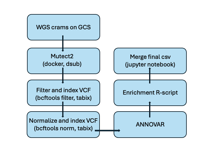
Note : Normalization here refers to standardizing VCF files using bcftools norm.
QC for CHIP calls
A custom R-script filters and annotates the variants from sample data by comparing them against predefined lists of significant variants (whitelists). It classifies variants into categories such as missense, loss-of-function, or splice site based on their functions and gene details. The script then flags relevant variants for inclusion in further analysis or manual review and generates a summary of the findings. Four different files are generated as outputs:
- A file with the whitelist filter applied
- One ready for manual review
- one with variant count information for debugging
- one with all the pre-whitelist variants listed
More details regarding the R-script can be found here. QC for CHIP calls was done using the whitelist and manual review variants. QC for CHIP calls was perfomed in two steps.
Step 1 - Filtering combined variant dataset
1.1. Combining variant files together
This step combines individual sample file into a single dataframe.
E.g - Combining all manual variant files into a single csv
from io import StringIO

client = storage.Client(project="PROJECT_ID")
bucket = client.bucket("BUCKET_NAME")

prefix = 'FILE_PREFIX'
blob_list = client.list_blobs(bucket, prefix=prefix)
batch_size = 10000
dfs_batches = []
dfs_batch = []

for i, blob in enumerate(blob_list):
    if blob.name.endswith('.annovar.varsOI.manualreview.csv'):
        # Download the blob as a string
        data = blob.download_as_text(encoding="utf-8")

        # Split the data into lines
        lines = data.strip().split('\n')

        # Read the first header line to get column names
        headers = lines[0].strip().split(',')

        # Determine the number of columns
        num_columns = len(headers)

        #Read CSV into DataFrame
        df = pd.read_csv(StringIO(data), header=None,  skiprows=1, names=headers)

        # Add the dataframe to the current batch
        dfs_batch.append(df)

        # If the current index is a multiple of the batch size, concatenate
        # the dataframes in the current batch and append the
        # result to the list of batches
        if len(dfs_batch) == batch_size:
            dfs_batches.append(pd.concat(dfs_batch))
            dfs_batch = []

# If there are any remaining dataframes in the current batch,
# append and concatenate them to dfs_batches
if len(dfs_batch) > 0:
    dfs_batches.append(pd.concat(dfs_batch))

# Concatenate all the batches into one dataframe
annovar_104k_varsOI_manualreview_csv = pd.concat(dfs_batches)
annovar_104k_varsOI_manualreview_csv.columns = [col.strip('"') for col in annovar_104k_varsOI_manualreview_csv.columns]
annovar_104k_varsOI_manualreview_csv.head()
1.2. Depth based flagging
We use the manual review and whitelisted variants moving forward, to perform the depth based filtering. The script is built to analyze and annotate variant data by applying a set of quality control checks, primarily focusing on read depth and strand representation. It processes two input files (whitelist and manual review variants), each containing variant calls with annotation details. The script extracts metrics such as total read depth, allele-specific depth, and strand information, classifies each variant based on its allelic structure (biallelic vs. multiallelic), and then applies a series of filters to flag variants that meet specific quality thresholds. The end result is an easily interpretable dataset that retains the original information but includes additional flags to indicate variant reliability.
To prepare our variant data for analysis, we start by unpacking key details like genotype, read depth, and strand direction from a single column. This helps break down complex sequencing information into separate, easy-to-use features. Next, we apply quality checks to make sure our variants are reliable. For each variant, we look at how many sequencing reads support it, whether the coverage is deep enough, and if both DNA strands show evidence of the variant.
What are the different outputs and what do they contain?
For each input file a corresponding file (*_variants_flagged.csv) that includes all original variant data along with several new columns representing the applied flags is produced. These outputs are useful because they not only show what variants were detected, but also how well-supported each one is.
For brevity, omitting full code here - Complete implementation is available here.
Step 2 - Idenitfying putative CHIP variants
2.1. Load baseline data
Baseline data has information from various sources - Demographics, Phecodes, Y/N for heamatological cancer and genotype information for the TERT promoter SNP (chr5:1285859). The individual sources are merged using the ship id for each sample.
phecodes_demographics_shipid= pd.merge(
phecodes_shipid_df[['shipping_id','phe_201','phe_202','phe_202_2','phe_204',
'phe_204_1','phe_204_12','phe_204_2']],
gia_phenotype_df[['shipping_id','age_blooddraw','sex','hare','gia','phenotype']],
on='shipping_id',
how='inner'
)

print("Number of samples after merging phecodes and demographics = "
,len(phecodes_demographics_shipid))
phecodes_demographics_shipid.head()
2.2. Manually reviewing variants for specific genes
The variants that need to be manually reviewed are grouped on the basis of three specific genes: DNMT3A, KIT, and MPL. This is then filtered to identify variants that match a known list of important mutations for each gene.
For each gene, we check if any of the known mutations appear in the NonsynOI column, which captures nonsynonymous mutations. If no matching mutation is found, the entry is marked as NA. The filtered list of variants is then saved for next steps.
# Define the mutation lists for DNMT3A, KIT, and MPL genes
dnmt3a_muts = ['F290I', 'F290C', 'V296M', 'P307S', 'P307R', 'R326H',....]
kit_muts = ['ins503', 'V559A', 'V559D', 'V559G', 'V559I', 'V560D',....]
mpl_muts = ['S505G', 'S505N', 'S505C', 'L510P', 'del513', 'W515A',....]

# Read in manual review variant list
manual_review_raw = pd.read_csv('/PATH/manual_review_variants.csv')
manual_review_raw.head()

# Filter the dataset based on the gene and mutation conditions
manual_review_passing = manual_review_raw[
    # Filter for DNMT3A, KIT and MPL mutations
    ((manual_review_raw['Gene.refGene'] == 'DNMT3A') & manual_review_raw['NonsynOI'].isin(dnmt3a_muts)) |
    ((manual_review_raw['Gene.refGene'] == 'KIT') & manual_review_raw['NonsynOI'].isin(kit_muts)) |
    ((manual_review_raw['Gene.refGene'] == 'MPL') & manual_review_raw['NonsynOI'].isin(mpl_muts))
]

# Summary of filtered data
print(manual_review_passing.info())
manual_review_passing.head()
2.3. Flagging germline variants
Pre-flagged (from step-1) and manual review variants are merged into a single dataset to create a comprehensive list for downstream analysis. Each row is a variant with associated metadata, read depth, annotations, etc.
# Read in pre-flagged variants
whitelist_raw = pd.read_csv('/PATH/annovar_104k_varsOI_wl_variants_flagged.csv')
whitelist_raw.head()

# Concatenate pre-flagged and manual review variants
vars_seq_flagged = pd.concat([whitelist_raw, manual_review_passing], ignore_index=True)
vars_seq_flagged.head()
2.4. Assessing allelic imbalance using binomial testing
We define a custom binomial p-value function to evaluate allele balance for each variant, testing whether the observed allele depths deviate significantly from the expected 50:50 ratio. Under the null hypothesis (which assumes equal representation of both reference and alternate alleles) the binomial distribution models the probability of observing the given counts. The p-value quantifies how likely such an imbalance would occur by chance; a low p-value indicates significant deviation from balanced allelic expression, suggesting potential technical or biological bias.
# Calculate two-tailed binomial p-value to test if allele balance deviates from expected - null hypothesis (default = 0.5 for 50:50 balance)
# Parameters:
  # a (int): Count of one allele (e.g., alt allele count)
  # b (int, optional): Count of the other allele (e.g., ref allele count)
  # n (int, optional): Total count (a + b). If not provided, it’s inferred
  # null_prob (float): Expected probability under null hypothesis

from scipy.stats import binom
def binom_p_val(a, b=None, n=None, null_prob=0.5):
if b is None:
b = n - a
if n is None:
n = a + b

# Two-tailed p-value:
p_val = 2 * binom.cdf(min(a, b), n, null_prob) - (a == b) * binom.pmf(a, n, null_prob)
return p_val
We start by cleaning the dataset, removing irrelevant columns and converting depth (DP), allele frequency (AF), allele depth (AD), and strand-specific counts (F1R2, F2R1) into usable formats. These fields are then split into lists and sorted to focus on the most prominent signals, such as the maximum allele frequency (maxAF).
To quantify imbalance, we apply a binomial test to each allele count. The test compares observed values against the null hypothesis of equal allele representation (50% each), returning a two-tailed p-value that captures the likelihood of such an imbalance arising by chance. The result is a clean, annotated dataset where each variant includes the most imbalanced allele frequencies and their statistical significance.
# Step 1: Select columns and remove those that start with "Other"
vars_seq_flagged = vars_seq_flagged.loc[:, ~vars_seq_flagged.columns.str.startswith('Other')]

# Step 2: Convert DP to numeric and split relevant columns into lists
vars_seq_flagged['DP'] = pd.to_numeric(vars_seq_flagged['DP'], errors='coerce')

# Ensure that AF, AD, F1R2, F2R1 are treated as strings and handle NaN values
vars_seq_flagged['AF'] = vars_seq_flagged['AF'].fillna('').astype(str)
vars_seq_flagged['AD'] = vars_seq_flagged['AD'].fillna('').astype(str)
vars_seq_flagged['F1R2'] = vars_seq_flagged['F1R2'].fillna('').astype(str)
vars_seq_flagged['F2R1'] = vars_seq_flagged['F2R1'].fillna('').astype(str)

# Step 3: Split the columns into lists
vars_seq_flagged['AF_list'] = vars_seq_flagged['AF'].str.split(',')
vars_seq_flagged['AD_list'] = vars_seq_flagged['AD'].str.split(',')
vars_seq_flagged['watson_list'] = vars_seq_flagged['F1R2'].str.split(',')
vars_seq_flagged['crick_list'] = vars_seq_flagged['F2R1'].str.split(',')

# Step 4: Sort the lists and calculate maxAF for each row
def sort_descending(x):
    return sorted(map(float, x), reverse=True)

vars_seq_flagged['AF_list'] = vars_seq_flagged['AF_list'].apply(sort_descending)
vars_seq_flagged['AD_list'] = vars_seq_flagged['AD_list'].apply(sort_descending)

# Step 5: Calculate maxAF
vars_seq_flagged['maxAF'] = vars_seq_flagged['AF_list'].apply(lambda x: max(x))

# Step 6: Apply binom_p_val to AD_list and DP (This step requires the correct handling)
def calc_binom_ps_05(row):
    # binom_p_val function expects a single value `a` and a total `n`
    # Here, `row['AD_list']` is a list, so we assume it's the list of alleles
    # We apply binom_p_val for each value in AD_list
    return [binom_p_val(a=val, n=row['DP'], null_prob=0.5) for val in row['AD_list']]

# Step 7: Apply binomial p-value
vars_seq_flagged['binom_ps_05'] = vars_seq_flagged.apply(calc_binom_ps_05, axis=1)

# Step 8: Store the result into variants_w_binom_ps
variants_w_binom_ps = vars_seq_flagged

# Step 9: Display DataFrame info (equivalent to glimpse in R)
print(variants_w_binom_ps.info())
variants_w_binom_ps.head()
2.5. Identifying mutation hotspots
To uncover potential mutation hotspots we group variants by their gene, genomic coordinates (Start, End), and mutation type (NonsynOI). Next, we group identical events and count how many times each unique mutation occurs across samples. These counts are stored in a new column. We then apply a threshold - any mutation that appears more than 15 times is considered a hotspot candidate and flagged as potential mutation hotspots.
2.6. Highlighting genes with mutation hotspots
After identifying mutation hotspots, the next step is to understand which genes are most commonly affected. We start by counting how many hotspots are found in each gene. This helps us see which genes keep showing up with multiple flagged mutations. The result is a ranked list where genes at the top are the ones most frequently affected by hotspots, as represented by the count.
Why is this useful?
Genes that appear often in the list might be important CHIP drivers and would require further investigation.
Most of the mutaions we have identified are in DNMT3A, as expected. We have some in TET2 and some in ASXL1 - this seems to be a tricky one as it could have both real mutations and artifacts. PDS5B is an artifact. Other genes require further investigation.
| Gene | No of hotspots identified |
|---|---|
| DNMT3A | 26 |
| TET2 | 13 |
| ASXL1 | 8 |
| SF3B1 | 7 |
| PPM1D | 5 |
| SRSF2 | 3 |
| PDS5B | 2 |
| CREBBP | 2 |
| PRPF8 | 2 |
| SETDB1 | 2 |
| STAG2 | 2 |
| TP53 | 2 |
| IDH2 | 1 |
| JAK2 | 1 |
| NF1 | 1 |
| RAD21 | 1 |
| GNB1 | 1 |
| GNAS | 1 |
2.7. Identifying predictors of CHIP mutations through logical regression
We are running a logistic regression model to predict whether a sample has a variant at a particular hotspot or not.
Two main questions are asked here:
Q1. Are the people who have this variant generally older (or younger) than those who dont?
Q2. Are the people with the TERT promoter SNP more (or less) likely to have the mutation?
The regression model we are running will return a p-value. If the estimated effect is positive, we will get an actual p-value. If the estimated effect is negative we will get 1. In other words, a small p-value (<0.05) indicates that there is statistical evidence that the predictor (Age/TERT SNP) is assocaited with the presence of that variant in that hotspot. A high p-value indicates that the predictor does not help in explaining why some people have that specific mutation.
Results for Logistic regression:
Output message - Regression failed: Perfect separation detected, results not available
Understanding what perfect seperation means:
The error “Perfect separation detected, results not available” means that your logistic regression model has encountered a situation where the predictor variable (e.g., age_blooddraw) perfectly predicts the outcome (CHIP variant - being 1 or 0). This causes the model to fail to converge, because the likelihood function goes to infinity and standard estimation techniques fail.
In logistic regression, we are modeling the probability of an outcome (having a CHIP variant). If the model sees that all individuals with a certain value of the predictor have the variant, and all others do not, it creates a situation like the below table:
| age_blooddraw | CHIP variant |
|---|---|
| 70 | 1 |
| 72 | 1 |
| 74 | 1 |
| 30 | 0 |
| 28 | 0 |
Here, the model “learns” that age perfectly separates the two classes — i.e., if age > 60 is always 1. Logistic regression tries to estimate probabilities between 0 and 1, but in this case, the estimated probabilities go to 1 or 0 exactly, which breaks model.
Alternate approaches
-
Check for any missing value with age : Was able to identify and remove 33 missing values within age values.
-
Check how age is distributed across age groups
phecodes_demographics_shipid.groupby('has_chip')['age_blooddraw'].describe()
| CHIP | count | mean age | std age | min age | 25% | 50% | 75% | max age |
|---|---|---|---|---|---|---|---|---|
| 0 - No | 102406 | 65.6 | 13.0 | 20.0 | 59.0 | 65.0 | 74.0 | 101.0 |
| 1 - Yes | 41 | 71.3 | 12.9 | 46.0 | 62.0 | 74.0 | 83.0 | 91.0 |
Key Takeaways:
-
Age difference: People who have the CHIP mutation (has_chip == 1) tend to be older on average than those who do not have the mutation. The mean age for individuals with the mutation is about 71 years, while for those without it, it’s 65 years.
-
Age distribution: The age distribution for people with the mutation (has_chip == 1) is more concentrated in the older age range (with a median of 74 years) compared to those without the mutation (median of 65 years).
-
Sample imbalance: There is an imbalance in the number of individuals in each group: 102,406 people without the mutation versus only 41 people with the mutation. This imbalance can affect statistical analysis, and special techniques (like over-sampling, under-sampling, or using weights) might be necessary to avoid biased results.
-
Skewed data: The higher median and age distribution for people with the mutation suggest that the mutation is more likely to occur in older individuals.
Conclusion
We have successfully completed CHIP variant calling for WGS release2 samples. Initial quality control results are promising — Alex and team have confirmed the presence of several CHIP variants within our dataset. The current list of putative variants has been shared with Caitlyn for further review to help identify additional true positive mutations. Next steps will focus on downstream analyses, including modeling the association between CHIP variant presence and key predictors - the TERT promoter SNP, and hematologic cancer.
Work in progress
-
Updating Y/N for hematologic cancer Within the phecodes_demographics_shipid dataset, check each sample for the presence of values in any of the selected hematologic cancer-related phecode columns. If a sample has a value (i.e., is coded) for at least one of these phecodes, label the sample as “Y” in a new column called has_hematologic_cancer. Otherwise, label it as “N”.
-
TERT promoter snp genotype Compute the total number of alternate alleles by summing the two values in a genotype string (e.g., “0/1” becomes 1, and “1/1” becomes 2). This gives us a quick way to understand how many copies of a variant an individual carries. If the genotype data is missing we treat he result is recorded as NA.
Join the discussion here !