#29 GWAS results for Data Release 2
Blog #29: GWAS results for Data Release 2
Background
In my last blog post I showed the methods devised to run PCA analysis in order to generate PCs to be used as covariates in GWAS analysis. Preliminary GWAS results for all combined samples and the European population were also described, in addition to early stages of GWAS comparisons across Data Releases 1 and 2. In the subsequent sections, I will present the results of the progress for GWAS within all populations and the correlation between both data releases.
GWAS
GWAS analysis, against a height phenotype, was run across all four population groups, in addition to the entire sample set. QQ Plots for the full sample set(Fig. 1), as well as the four population subsets(Fig. 2), show an increased lambda as the total number of samples increases above a certain threshold.
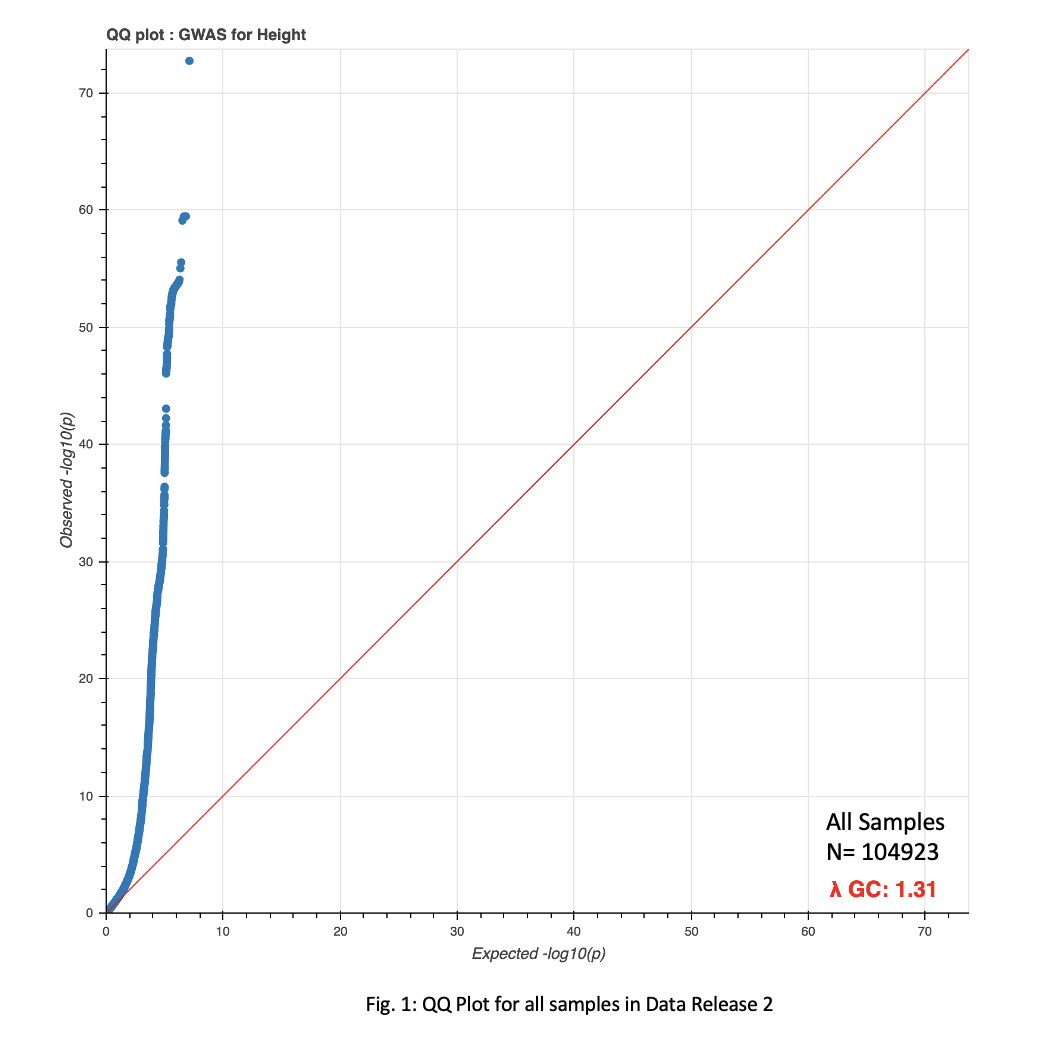
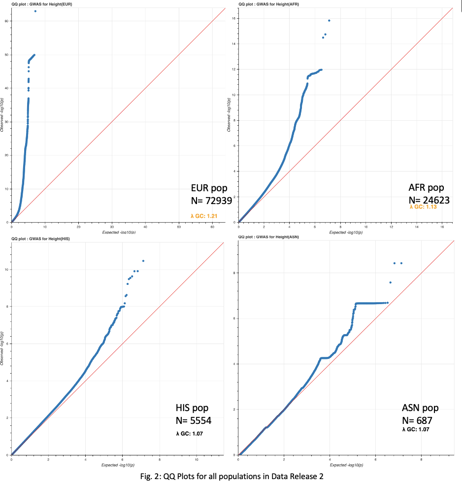 A P-value of 5e-8 was implemented as a cutoff for significant loci. This cutoff resulted in 17,738, 15,587, 541, 33, and 3 loci for the total sample set, European, African, Hispanic, and Asian populations, respectively(Fig. 3-4).
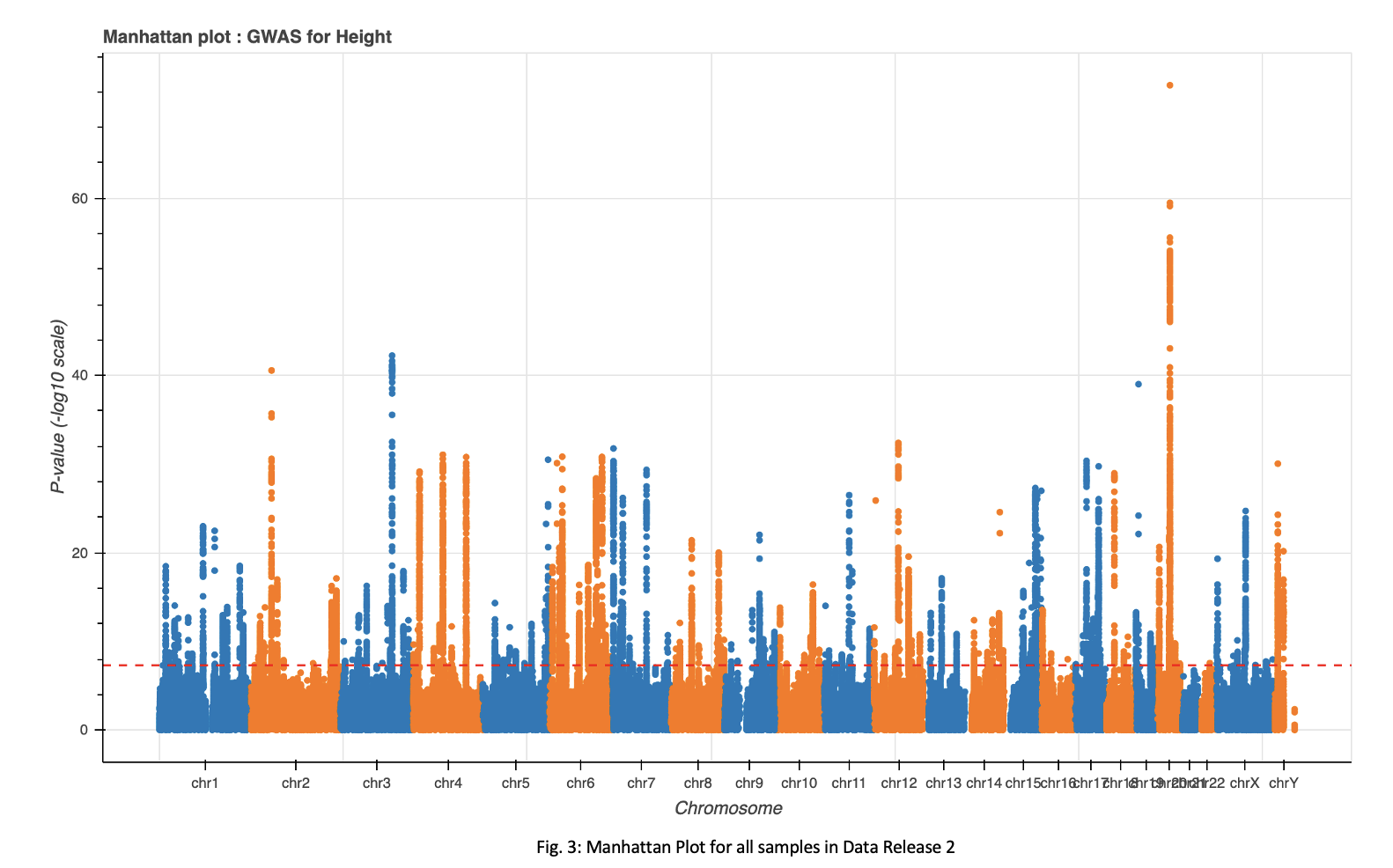
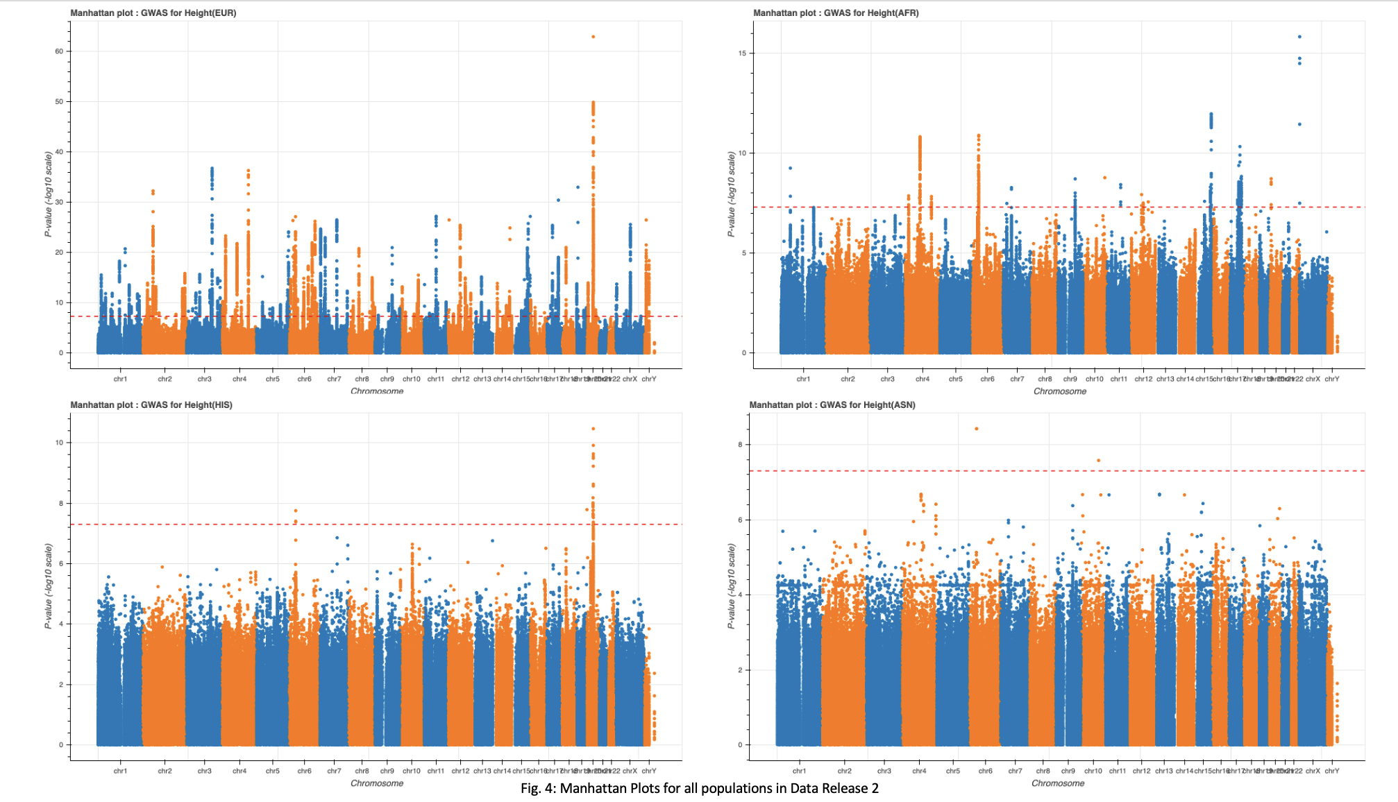
The full dataset and European subset showed an extremely high number of significant loci. Upon seeing this, I implemented a more stringent cutoff for these two groups. Increasing the cutoff to 5e-9 resulted in a count of 13,049 and 11,467 significant loci for the full dataset and European population, respectively. These numbers remain high and may require further exploration.
Analysis of the top ten loci in both the full dataset and the European population groups show multiple hits to genes UQCC1 and GDF5(Table. 1), both of which are implicated in regulation of height.
Comparison between Data Release 1 and Data Release 2
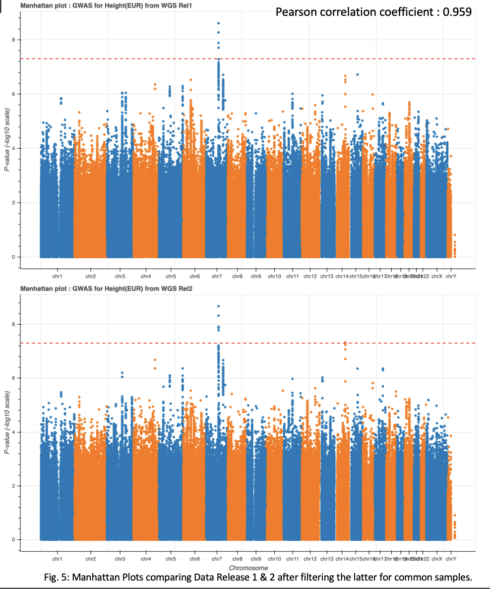
In my last blog I also discussed the early stages of comparing the GWAS results across Data Releases 1 and 2. Initially, I filtered GWAS results for Data Release 2 to only include samples in common with the first release. This method resulted in very little correlation between the two datasets. I have since changed my strategy by filtering common samples prior to running GWAS, which has resulted in much better overlap. Filtering of dataset 2 resulted in 10,385 samples compared to 10,390 samples in Data Release 1.
When testing overlapping variants, both datasets indicate high correlation. This is indicated by a Pearson correlation score of 0.958587(Fig. 5) I also observed high overlap between significant loci for both the full data set and the European population group, using a cutoff of 5e-8 (Fig. 5, Table. 2, & Table. 3). These results indicate that the aggregation and filtering methods used in data generation, as well as the PCA methodology implemented, are valid.
Future steps
- Polish GWAS figures
- Remove samples with no assigned ethnicity from PCA scatterplot
- Fix chromosome title overlap on X axis of Manhattan plots
- Add 5e-9 line to relevant Manhattan plots
- Novel variant discovery using hail methods
- I have been working to format a list of known SNPs attained from NCBI. Some hiccups involved in this process included formatting the file to load into hail, filtering contigs to only include the autosomes and two sex chromosomes, changing contig names to match that of our reference, and formatting the locus and allele fields to a usable format in Hail. Only the latter remains to be completed. Once done, a join between our genotype table and this table may reveal novel variants.
Discuss
Join the discussion on our GitHub