#47 CHIP calling - Pipeline modifications and Cost estimation
CHIP calling
Mutect2, a variant caller from the GATK suite of tools, was implemented on GCP to identify CHIP mutations from 10k WGS samples using the broadinstitute/gatk:latest docker image. This paper describes the CHIP calling on WGS data in more detail.
Mutect2 successfully processed 9994 WGS samples, with a few samples still being reviewed to resolve processing issues. All other steps, including filtration, indexing, ANNOVAR, and enrichment, were executed on an n1-standard-4 VM.
Post ANNOVAR, each sample is run through a R-script which filters out high quality variants. The script generates four distinct csv files for each sample. These outputs were merged into a single consolidated csv for each output type using jupyter notebook (Python 3.10.4. Packages used - google.cloud.storage pandas matplotlib seaborn). Additionally, SHIPids were anonymized and standardized across all files (e.g., “sample1” consistently represents the same SHIPid across all 4 files) before being shared with collaborators.
Pipeline modifications
1. Modifying the minimum depth during filtration
Initially we went with the original script used by Alex and team which filters variants with a depth of coverage (DP) less than 20 (MIN(FORMAT/DP)<20), along with filtering out variants where both the forward and reverse reads have low mapping quality scores, typically less than 1 (MIN(FORMAT/F1R2)<1) || (MIN(FORMAT/F2R1)<1).
Although these results looked promising, given the sequencing depth is ~30x and the variants ranged from DP 20-64 in the results, a DP >= 15 was suggested to help us detect larger CHIP clones and improve sensitivity.
2. Revised sequence of steps
After our initial discussions, we planned to execute the pipeline on GCP in the following order: Mutect2, filtration and indexing, merging and normalization, ANNOVAR, and then enrichment of CHIP calls.
However, upon further review, we determined that it would be more effective to merge the output files after completing ANNOVAR and enrichment steps. This adjustment changes the pipeline workflow and the number of output files produced at each stage. The decision to modify the pipeline was based on two key reasons:
-
By default, the R-script used for enrichment processes each sample individually to produce four distinct output files. As a result, while it is possible to use a single merged file, doing so would not provide a list of variants specific to each sample.
-
Although we could modify the R-script to read sample names from a merged file (as initially planned), the file itself lacks sample information (SHIPid), again leading to the same problem of not being able to idenitfy sample specific variants. Thus, we opted to perform the merging (i.e. appending the results from 9994 samples in to one csv file) after generating the list of variants for each sample.
2.1. New CHIP pipeline
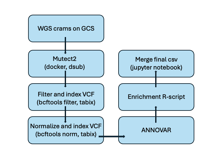
Note : Normalization here refers to standardizing VCF files using bcftools norm.
The process of Mutect2, filtering and indexing are explained in detail in this blog post.
2.2. ANNOVAR outputs
There are two steps in ANNOVAR:
- Step 1 : Convert the variant information from the normalized VCF file into a format compatible with ANNOVAR. This generates a .log and a .input file for each of the samples, which is used a input for the next step.
#!/bin/bash

# Define paths for I/O files
OUT_DIR="/PATH/"
IN_DIR="/PATH/"

# Ensure the output directory exists
mkdir -p "$OUT_DIR"

echo "Generating annovar inputs from vcfs.."

# Loop through each .vcf.gz file in TEMP_DIR
find "$IN_DIR" -name "*.vcf.gz" | while read -r file; do
    base_name=$(basename "$file" .vcf.gz)

    # Run convert2annovar.pl
    perl /PATH/convert2annovar.pl -format vcf4 "$file" \
        -outfile "$OUT_DIR"/"$base_name"_annovar.input \
        -allsample -withfreq -include \
        2> "$OUT_DIR"/"$base_name"_annovar.log
done
- Step 2 : Annotate the converted VCF file with functional information. This generates a .multianno.txt file for each sample, which are subsequently used as inputs for the enrichment step. Each output file is prefixed with the correponding SHIPid as required by the R-script.
#!/bin/bash

# Directory where input files (*.annovar.input) and logs (*.annovar.log) are stored
OUT_DIR="/PATH/"

# Ensure the output directory exists
# mkdir -p "$OUT_DIR"

echo "Running annovar step 2.."

# Find all *.norm_annovar.input files in OUT_DIR and process them in parallel
find "$OUT_DIR" -maxdepth 1 -type f -name "*.norm_annovar.input" |
\ parallel --jobs 4 --eta \
        'base_name=$(basename {} .norm_annovar.input); \
         perl /PATH/table_annovar.pl \
            {} \
            /PATH/annovar/humandb/ \
            -buildver hg38 \
            -out '"$OUT_DIR"'/${base_name}_annovar_output \
            -remove \
            -protocol refGene,knownGene,cosmic70 \
            -operation g,g,f \
            -nastring . \
            -otherinfo \
            2>> '"$OUT_DIR"'/${base_name}.norm_annovar.log'

echo "All files processed."
2.3. Enrichment of variants
The R-script filters and annotates the variants from sample data by comparing them against predefined lists of significant variants (whitelists). It classifies variants into categories such as missense, loss-of-function, or splice site based on their functions and gene details. The script then flags relevant variants for inclusion in further analysis or manual review, and generates output files summarizing the findings. Finally, it creates separate files for all variants, those in the whitelist, and those flagged for manual review. More details regarding the R-script can be found here.
I’m currently updating this notebook to include further analysis and detailed decriptions. In the meantime, feel free to review the work that’s already done.
Cost estimation for running Mutect2 (n = 10)
A cost analysis for running Mutect2 on GCP for a small subset of 10 samples has been shown below. Cost was computed using the pricing calculator for a n1-standard1 machine type with a boot disk size of 10GB.
| Sample | CPU time (min) | Cost CPU time (USD) | Wall clock time (min) | Cost wall clock time(USD) |
|---|---|---|---|---|
| S1 | 2.00 | 0.05 | 6.00 | 0.14 |
| S2 | 2.04 | 0.05 | 6.55 | 0.16 |
| S3 | 2.11 | 0.05 | 6.21 | 0.15 |
| S4 | 1.81 | 0.04 | 6.09 | 0.15 |
| S5 | 1.62 | 0.04 | 5:01 | 0.12 |
| S6 | 2.06 | 0.05 | 6:10 | 0.15 |
| S7 | 1.94 | 0.05 | 5:00 | 0.12 |
| S8 | 1.74 | 0.04 | 5:45 | 0.13 |
| S9 | 1.79 | 0.04 | 6:00 | 0.14 |
| S10 | 1.93 | 0.05 | 5:54 | 0.13 |
Note:
CPU time - represents the total amount of time that the CPU spends actively processing the task. It does not include time when the CPU is idle or waiting, such as during I/O operations, network delays, or when the VM is waiting for resources.
Wall clock time - This is the real-world elapsed time from the start to the end of a task or process. It includes all time intervals, such as CPU processing time, waiting time, and any other delays that might occur during execution.
CHIP outputs
Average files sizes for the output files at various stages are mentioned below for the the 9994 WGS sample set. I took into account Joe’s feedback from our previous lab meeting regarding file size labeling on GCP. Files were labeled as Kb, which stands for Kibibytes (Kib). To convert these to Kilobytes (KB), you multiply by 1.024, and to convert to Megabytes (MB), you divide by 1024. All the values provided above have been converted to MB.
-
Mutect 2 dsub job output (Number of files produced = 9994)
VCF files – 271.78 MB -
Filtration for depth (Number of files produced = 9994 * 2 = 19,988)
Filtered VCF 28.51 MB, Indexed filtered vcf – 3.59 MB -
Normalization of filtered files for annovar (Number of files produced = 9994 * 2 = 19,988)
Normalized vcf – 28.65 MB, Indexed normalized vcf – 3.59 MB -
Annovar outputs (Number of files produced = 9994 * 3 = 29,982)
Anovar.log – 5.55MB
Annovar.input – 34.68 MB
Annovar_hg38_multianno.txt – 80.28 MB -
Enrichment Rscript output files (Number of files produced = 9994 * 4 = 39,976)
File1.csv – 36.43 MB
File2.csv – 0.54 MB
File3.csv – 0.10 MB
File4.csv – 0.67 MB -
Merging post enrichment for each file type (actual file sizes, not average. Number of files produced = 4)
File1_10k.csv – 325.30 MB
File2_10k.csv – 0.11 MB
File3_10k.csv – 0.17 MB
File4_10k.csv – 1.25 MB
The most crucial files are the VCFs from Mutect2, the ANNOVAR outputs, and the merged csvs after enrichment. The remaining files (from filtration, normalization, and enrichment) can be regenerated, as the scripts used for these steps do not take much time to run (~10 mins for 10k samples) on a n1-standard4 VM.
I have completed the 10k run after modifying the filtration script to filter for variants with DP>15. The results were shared with Alex and team after anonymizing the SHIPids. The results look promising with minimal artifact introduction. Caitlyn (who has been our point person) was also able to identify 15 new variants with the lower DP threshold. The next step would be to expand the study to the remaining samples form WGS Release2.
Next steps
- Update git repo with new CHIP calling scripts, cost estimation sheet and analysis notebook.
- Update GCS folders with corresponding README.md files explaining output files and how to create intermediate files.
- Scale up CHIP pipeline for the reamining samples from WGS DR2.
Join the discussion here!